Chapter 5 Population Regulation and Stochasticity
Although Turchin’s law is often observed for short periods of time, eventually it always breaks down. Why? Under what conditions does exponential growth (or decay) come to a halt, and can we predict those conditions in advance?
Pheasants on the Island
8 pheasants were released on Protection Island in 1937 (Einarsen 1945). The pheasants were counted twice a year until the entire population was eaten in 1943 when troops were posted to the island (fact check this – not mentioned in Einarsen 1945)! There were 30 pheasants in 1938, so using equations from Chapter 4 we can work out the annual rate of growth assuming the population grows exponentially:
\[ r=ln\left(\frac{N_t}{N_0}\right)/t = ln\left(\frac{30}{8}\right)/1 = 1.32 \] which is an extremely high rate of growth. The line in Figure 5.1 shows the projected population size assuming this growth rate continued through 1943. Clearly, from 1941 on the population was growing at less than the exponential rate. Why did the growth rate slow down?
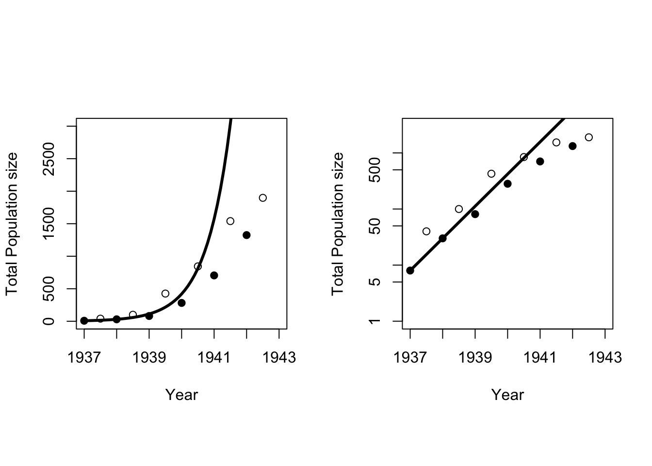
Figure 5.1: Total population size of pheasants on Einarsen Island. Filled circles are the spring counts, and open circles are the fall counts. The solid line is exponential growth with \(r = 1.32\). The panel on the right is on a logarithmic scale.
5.1 Resource Limitation
Although we’ll never know for sure, it seems likely that the Protection Island Pheasants stopped growing so fast because they were lacking some resource needed for growth, survival, or reproduction. Competition for resources, either intra-specific competition with other members of the same species, or inter-specific competition with members of a different species, can reduce the resources available to each individual. If the per capita rates of any of the processes in the fundamental equation (4.1) are affected by the amount of resources available to an individual, then this competition can reduce the population growth rate. Consider a simple example. There is a resource that is critical to reproduction, so the per capita birth rate is proportional to the amount of resource per individual. Individuals of the population compete with each other in scramble fashion, so the amount each individual obtains is a simple fraction of the total available. More individuals in the population equal less resources for each. This resource limitation leads to a reduction in the per capita rate of reproduction
\[\begin{equation} b\left(N\right)=\frac{a}{N} \tag{5.1} \end{equation}\]
where \(a\) is a parameter describing how the per capita birth rate changes with population size. The parameter \(a\) is readily interpretable as the per capita birth rate when there is exactly 1 individual in the population, in other words, in the absence of competition. In reality, we never see birth rates this large. However you can estimate it by observing how birth rates vary with population size. It is also possible to estimate it from life history data if we know the maximum limits of birth rates under ideal conditions. We can work out what the population consequences of this simple assumption are by substituting (5.1) into (4.1)
\[\begin{equation} N'=\left(\frac{a}{N}-d\right)N=\frac{aN}{N}-dN=a-dN \tag{5.2} \end{equation}\]
and assuming that immigration and emigration are zero.
Instead of a constant rate of growth, we have a rate of growth that decreases linearly with \(N\), the population size. That is, (5.2) is the equation of a line, with a y-intercept of a, and a slope of –d. When the population is small, the growth rate \(N'\) is positive, so the population grows. Eventually the population gets large enough that the growth rate \(N'\) becomes negative. Populations that large or larger will shrink because the population growth rate (\(N'\)) is negative. The point that divides populations that grow from populations that shrink is the x-intercept of our linear equation. The x-intercept is the value of \(N\) that yields \(N'\) = 0 when substituted into (5.2). We can find this value by setting (5.2) equal to zero, and solving for \(N\).
\[\begin{equation*} \begin{split} N'=a-dN & = 0 \\ dN & = a \\ N^* & =\frac{a}{d} \end{split} \end{equation*}\]
In mathematical terms, this point is called an equilibrium point, because if the population ends up exactly at \(N^*\), it will remain there indefinitely. It will stay there in the absence of other forces (sound familiar?) because the rate of change in \(N\) is zero at that point. In ecological terms, this point is known as the carrying capacity, the size of the population that can be supported by the present environment. This is also known as the ecological carrying capacity, and is also often given the symbol \(K\).
There’s another equilibrium point in this model. If a population reaches \(N = 0\), then the growth rate is 0 and the population will remain at that point indefinitely. However, it is not a stable equilibrium point, because any slight perturbation that makes \(N > 0\) will lead to positive population growth. This is quite different from the equilibrium point at \(N = K\). There positive perturbations to \(N\) lead to negative growth rates (birth rate lower than death rate see Figure 5.2), while negative perturbations to \(N\) lead to positive growth rates (birth rates higher than death rates). These feedbacks will tend to keep the population in the vicinity of the carrying capacity.
5.1 The many flavors of carrying capacity
The term carrying capacity gets used loosely in many population management contexts. In addition to the very specific sense of the population size at which the rate of change is zero, there is at least one other meaning that is important. The social carrying capacity is the maximum population size that is tolerable to human populations living in the same area. This term usually gets used in the context of over-abundant populations. A population is over-abundant when (at least some) humans feel there are too many of a species. This is an area that is fraught with potential for conflict. Inevitably, there will be groups of people that disagree on what the suitable population size is for a certain species. The most prominent example of this in the national news is the Northern Rocky Mountain population of grey wolves. Conservationists want more wolves, while ranchers and others that live in the vicinity want fewer – ideally no – wolves. The only place where wolves are likely to reach their ecological carrying capacity is in Yellowstone National Park. Outside the park, social pressure has lead to harvesting, which in turn will lead to lower population size.
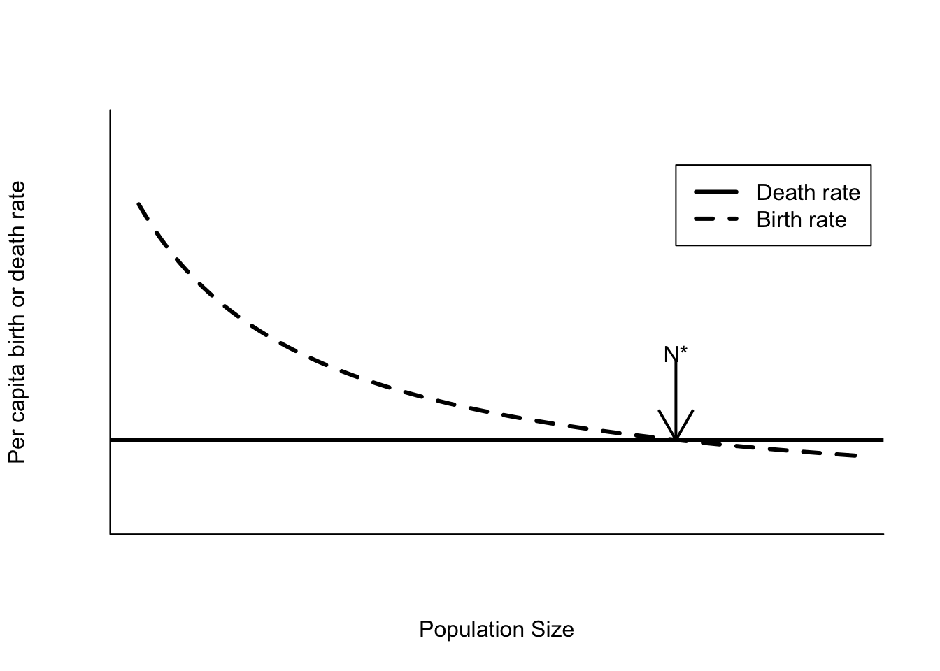
Figure 5.2: Per capita birth and death rates for a model with birth rates affected by scramble competition
So what do the dynamics of this model look like? Whether we start above or below \(N^*\), the population decays (grows) towards the equilibrium point (Figure 5.3). The important assumption here is that the parameters \(a\) and \(d\) are constant over time. The population growth rate changes as population size changes, but the relationship between growth rate and population size is constant. We say this population is regulated, because it neither grows towards infinity nor decays towards zero without limits.
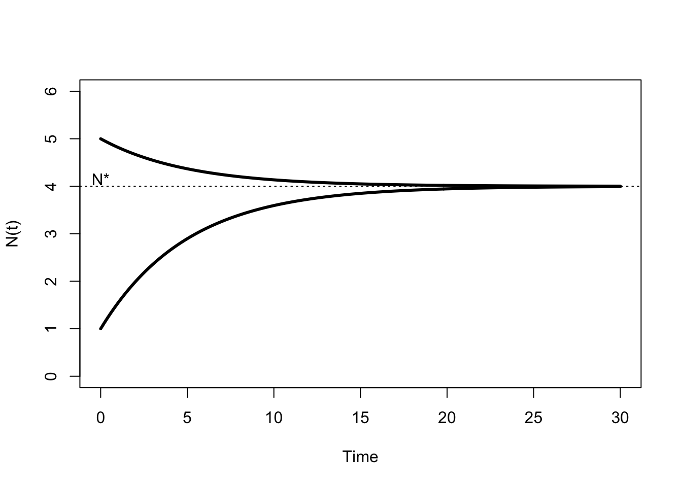
Figure 5.3: Growth trajectories implied by (5.2) for \(a=0.8\) and \(d=0.2\).
Early mathematical ecologists formulated models like (5.2), and referred to the relationship between population size and population growth rate as density dependence. As mathematicians, these early theoreticians were particularly fond of straight lines (the math is easier), and if both per capita death and birth rates are straight lines (Figure 5.4) then we obtain
\[\begin{equation} N'=rN\left(1-\frac{N}{K}\right) \tag{5.3} \end{equation}\]
where \(r\) is the intrinsic rate of population growth and \(K\) is the ecological carrying capacity. This is commonly known as the logistic equation. Pierre-Francois Verhulst first published this model in 1838 after reading Thomas Malthus An Essay on the Principle of Population (which also inspired Charles Darwin). It was “rediscovered” by Raymond Pearl and Lowell Reed in 1920, which is why you’ll sometimes see this described as the Pearl-Verhulst equation. Alfred Lotka published it in 1925 and called it the Law of population growth.
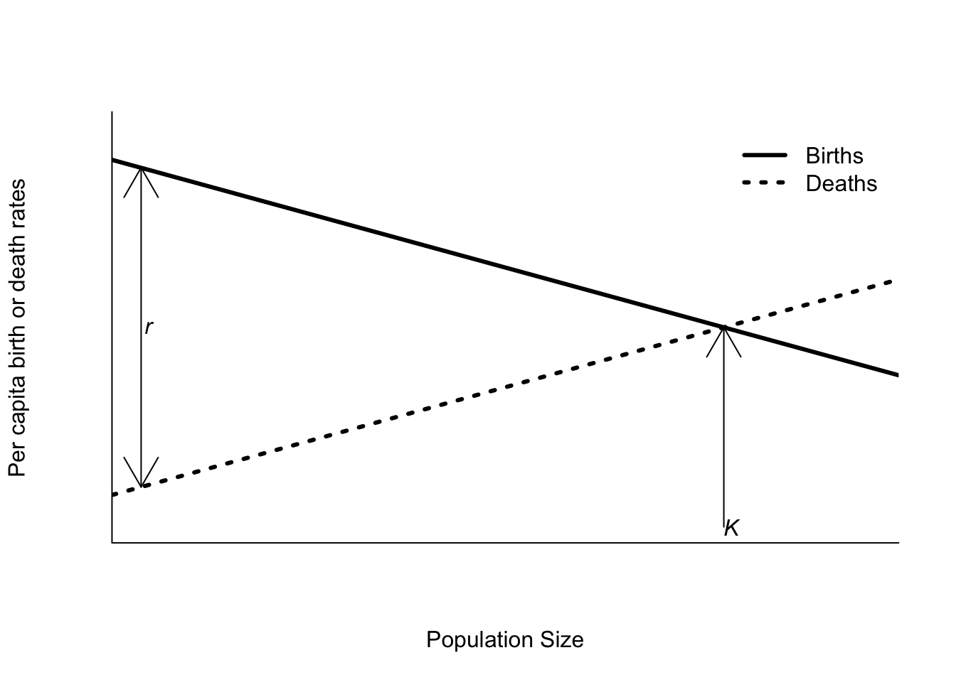
Figure 5.4: Per capita birth and death rates as functions of density as assumed by the logistic equation.
In the graphical depiction of the logistic equation (Figure 5.4), the carrying capacity \(K\) is given by the intersection of the two lines. The intrinsic rate of growth, \(r\), is the difference between the birth rate and death rate when the population size is zero, or simply the difference between the y-intercepts of both lines. The logistic equation is usually shown as I’ve done here, with both death and birth rates changing with population size. However, that’s not really essential. As long as the two lines cross at some positive population size, you will see logistic dynamics. So the per capita birth rate can be independent of density (ie. a flat line) as long as the per capita death rate is increasing. In addition, although it is common to talk about resource competition as the source of density dependence, it is not the only possibility. Changes in death rates can also arise from changes in predator behavior. If a biotic or abiotic process affects birth or death rates differently at different population sizes, it can lead to density dependent population growth.
The logistic equation (5.3) describes the rate of change in continuous time. This is mathematically convienent, but not necessarily a good approximation of population growth in temperate climates. Temperate climates, or seasonal climates, generally have very distinct periods when populations give birth, migrate, and die. In addition, it is easier to use these equations in discrete time (projecting one year from the previous year) in readily available software like R. Continuous time models require specialized software and/or great mathematical ability to obtain solutions. We need to move from (5.3) to something like
\[\begin{equation*} N_{t+1} = N_t f(N_t) \end{equation*}\]
where \(f(N_t)\) gives the net per capita rate of population growth. If \(f(N_t) = \lambda = e^r\), then we have simple geometric population growth, which is the discrete time version of exponential growth. If \(f(N_t)\) is not constant, but depends on \(N_t\), as in logistic population growth, we have to do something more complex. One approximation that works quite well is to assume that the population grows exponentially at a constant rate for the next time step (I’ll use 1 year as the time step). At the end of the year, the growth rate is reset to a new value determined by the new population size. That is, assume that the growth rate changes between years, but not within a year. In that case
\[\begin{equation} N_{t+1} = N_t f(N_t) = N_t e^{r\left(1-\frac{N_t}{K}\right)} \end{equation}\]
This is called the “Ricker equation” after the fisheries biologist that first worked it out. The dynamics of this equation for \(r<2\) are very similar to the continuous time logistic equation. The population steadily approaches \(K\) from above (if \(N_t > K\)) or below if (\(N_t < K\)). However, the dynamics of the Ricker equation have some extra wrinkles. For example, if \(r\) is large enough it is possible for \(N_{t+1} > K\) even though \(N_t < K\). In other words, the population can overshoot the carrying capacity. This leads to a series of oscillations around \(K\), which gradually damp down in amplitude (Figure 5.5). When \(r >= 2\) the dynamics of the Ricker equation become very bizarre. Wildlife populations will rarely have intrinsic growth rates that large, so we won’t worry about that now. From a practical perspective, the best property of the Ricker equation is that it will not predict future population sizes less than or equal to zero.
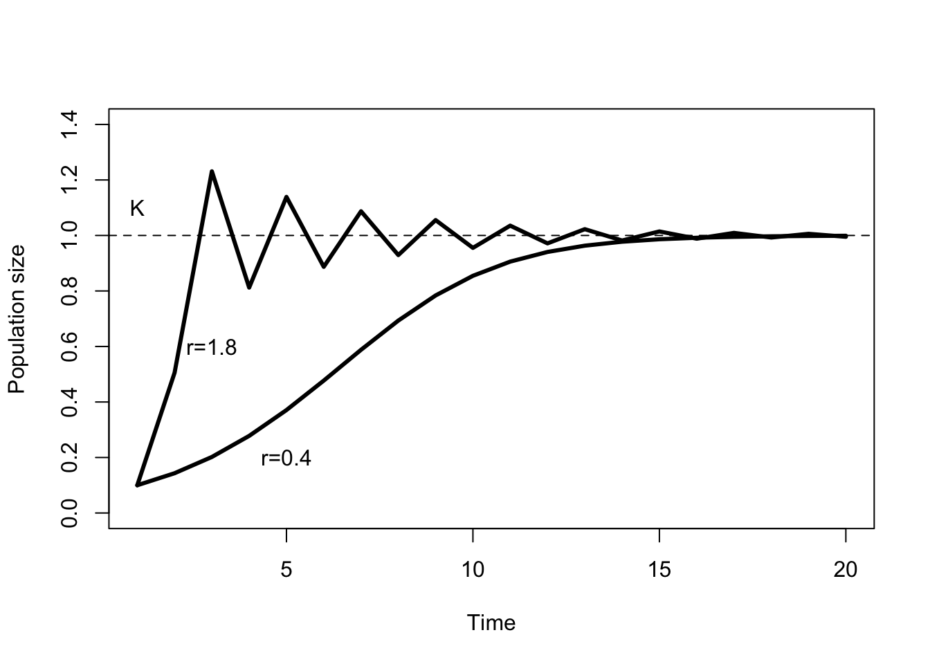
Figure 5.5: Behavior of the discrete time Ricker model for two different values of \(r\). \(K=1\) and \(N_0 = 0.1\).
5.2 Density Dependent or Independent?
The 20th century witnessed a vitriolic debate over the nature of population regulation. On the one hand were ecologists who thought that intraspecific competition led to changes in birth and death rates implied by the logistic equation. This was the “density dependent school,” epitomized by British ornithologist David Lack. Lack observed birds’ nests, and in particular the number of baby birds that successfully fledged. In the populations that he studied the number of fledgelings typically decreased with population size, and hence would lead to a regulated population as predicted by the logistic equation.
On the other hand were ecologists who thought that the effects of the environment, including weather and food resources, were paramount. This “density independent school” argued that populations were affected more by abiotic factors, and that the effects of these abiotic factors on populations did not depend on the population size. Herbert Andrewartha and Charles Birch, two Australian scientists who worked on insects, were the chief architects of this view. They had followed the numbers of thrips and aphids on a rose bush outside their office building for many, many years, and observed that the population size was strongly influenced by the amount of rainfall, and not by the population size in previous weeks. (That bush was outside my office when I worked at the Waite campus of the University of Adelaide. It still has thrips and aphids. There should be a shrine there.)
So who is right? To some extent, both camps are, but the density independent camp is more wrong. It is quite easy to show that a population that is subject to random shocks (ie. weather), but otherwise has a constant population growth rate \(r\), will eventually either decay to zero (if \(r<0\)) or grow to infinity (if \(r>0\)). In order for a population to persist at some finite size, the rate of population growth must eventually decrease with increasing population size. However, it does not have to exactly match the logistic equation. What confused many, many ecologists thoughout the 20th century was the derivation of the logistic function from the assumption that per capita birth and death rates were straight lines. This makes the math easy, but it isn’t necessary to have a regulated population. The functions \(b(N)\) and \(d(N)\) can, and do, have many different shapes (Figure 5.6). In particular, if there is a portion of the curve that is flat, then when a population is within that region birth rates remain constant with apparently no relationship to population size - density independence! However, if a population grows large enough, density dependence will, indeed must, appear.
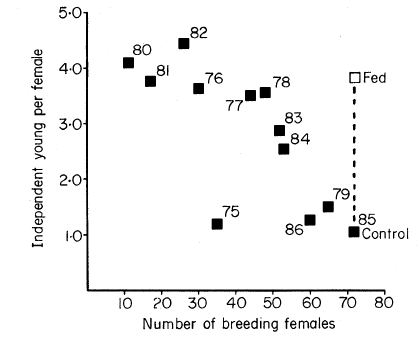
Figure 5.6: The mean number of independent young as a function of the number of breeding females in the Mandarte Island Song Sparrow population. In 1985 some females received supplementary feeding, which increased their reproductive output. The rate of change in reproductive output is lower, almost flat, when the number of females is less than 40. Adapted from Arcese and Smith (1988)
So in what sense were Andrewartha and Birch right? What they did was point out that the environment matters. The parameters in the logistic equation (or any other population model), \(r\) and \(K\), are not constant with time. Rather, they can vary randomly from one time period to the next. In other words the environment is stochastic.
5.3 Stochasticity
The word stochastic comes from Greek, where its original meaning was “to aim at a mark, guess” (OED online, Feb 17 2012). The modern meaning of a quantity “that follows some random probability distribution or pattern, so that its behavior may be analyzed statistically but not predicted precisely” did not come into use until the 20th century. In population dynamics the idea that the number of individuals in a population could be treated as a random variable in models can be traced to J.G. Skellam’s book chapter “The mathematical approach to population dynamics” in 1955 in The numbers of man and animals. Prior to this point stochastic variation in numbers was attributed to sampling error alone.
The fundamental process that makes population dynamics stochastic is that births and deaths occur at random. Not every individual female in a population gives birth to the same number of individuals in a period of time. Whether or not an individual dies is fundamentally not predictable. Instead, each of these events occurs with some probability. We call this source of stochasticity in populations demographic stochasticity.
Although physicists cannot predict the behavior of individual particles in a gas, the statistical properties of many, many particles in a container are quite predictable. For example, as the temperature of a gas in an enclosed container rises, so does the pressure (Ideal gas law). Similarly, ecologists cannot predict the fate of individuals but changes in the number of a whole group of individuals can be quite predictable. By analogy with the dynamics of particles, the larger the group, the more predictable the changes in group size. Demographic stochasticity has larger effects on smaller populations.
The development of an exponentially growing population with demographic stochasticity follows the development in Nick Gotelli’s book “A Primer of Ecology”. We’re now thinking of births and deaths as discrete events that occur sequentially. So a population might experience a sequence like BBDBDBBBDDBD over some short period of time. Alternatively, it could be DBBDDDBDBBBB. The point is that we now cannot predict exactly how many births or deaths will occur over some span of time. If the per capita birth rate, \(b\), is constant over time then the probability of a birth across any span of time is \(p(b)=\frac{b}{b+d}\), because we will either have a birth or a death. Similarly the probability of a death becomes \(p(d)=\frac{d}{b+d}\). As a result, we can no longer talk about the population size at time \(t\), but only about the statistical properties of the distribution of population size, the mean and the variance. The mean is easy - it is just the same formula as for exponential growth.
\[\begin{equation} \bar{N_t}=N_0 e^{rt} \tag{5.4} \end{equation}\]
Calculating the variance depends on whether or not \(b\) and \(d\) are equal. Usually they will not be equal, and then the variance of \(N_t\) is
\[\begin{equation} \sigma_{N_t}^2=\frac{N_0 \left(b+d\right) e^{rt}\left(e^{rt}-1\right)}{r} \tag{5.5} \end{equation}\]
There are several important things to notice about this equation. First, the variance increases with population size, as we’ve observed before (See box Taylor’s Law). This is different from sampling variation however – this is fundamental unpredictability about future population sizes. The variance also increases with the absolute magnitude of the per capita birth and death rates, because of the term \(b+d\). That is, a population with \(b=0.1\) and \(d=0.05\) will be less variable than a population with \(b=1.1\) and \(d=1.05\), even though both populations have a growth rate \(r=0.05\). The second population has much higher rates of turnover, and so a greater risk of a run of births or deaths causing the population to deviate from the average. Finally, the variance will increase with time, because of the terms containing \(e^{rt}\) (Figure 5.7). If the per capita birth and death rates are equal, \(r = 0\), and the variance is simply
\[\begin{equation*} \sigma_{N_t}^2=2 N_0 b t . \end{equation*}\]
In the presence of stochasticity, it is quite possible for populations with positive population growth rates to remain flat or even decrease periodically.
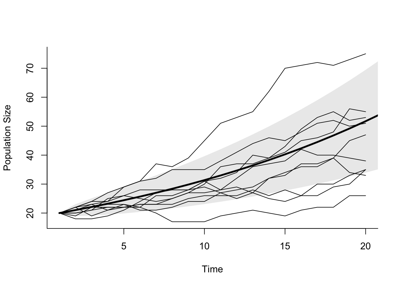
Figure 5.7: Exponential growth with demographic stochasticity. Thin lines are 20 replicate time series with \(N_0 = 20\), \(b=0.1\), and \(d=0.05\). The thick line is the expected population size, and the grey polygon shows the confidence limits on population size. Notice that trajectories can be above or below the average.
The model in (5.4) assumes that the per capita birth and death rates remain constant across time. We know that is not true; some years are wet, some dry. Some years are hot, others cold. In some years predators are abundant, while in a couple of years they may be much less abundant. To account for this variability statistically, we can think of the per capita rates \(b\) and \(d\) as stochastic; that is, their values follow some probability distribution so that the statistical properties are known, even if the particular rates for a particular year are not predictable.
Consider a population of northern Bobwhites (Colinus virginianus). We know that in years with particularly cold winters with late deep snow, Bobwhites have very low survival (Figure 5.8). These sorts of years do not occur often, but when they do they have a big effect on the dynamics of the population. We can have a death rate in good years, \(d_{good} = 0.2\), and a death rate in bad years \(d_{bad} = 0.8\). In order to predict the dynamics of this population on average, we also need to know the probability that a bad year occurs, let us call that \(p_{bad} = 0.05\), so that bad years happen, on average, once every 20 years.
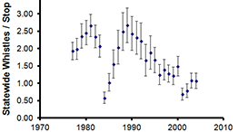
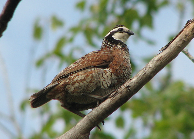
Figure 5.8: The mean number of whistles per stop over time for Northern Bobwhite (Colinus virginianus) in Nebraska. 1983 was a very late, hard winter with deep snow. Image courtesy of noflickster, creative commons attribution, noncommercial, sharealike.
## Warning in rbar * t: Recycling array of length 1 in array-vector arithmetic is deprecated.
##   Use c() or as.vector() instead.
## Warning in (b - d) - rbar: Recycling array of length 1 in vector-array arithmetic is deprecated.
## Use c() or as.vector() instead.## Warning in 2 * rbar * t: Recycling array of length 1 in array-vector arithmetic is deprecated.
## Use c() or as.vector() instead.## Warning in rsigma2 * t: Recycling array of length 1 in array-vector arithmetic is deprecated.
## Use c() or as.vector() instead.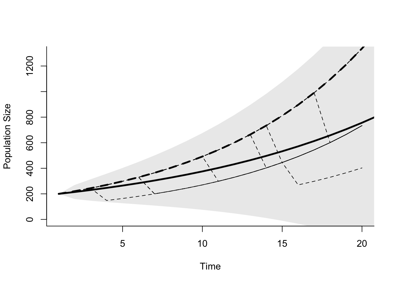
Figure 5.9: Exponentially growing population with environmental stochasticity. The dashed lines are 20 replicate simulations with \(b=0.3\) and \(d=0.2\) in 19 out of 20 years, and \(d=0.8\) in 1 out of 20 years. The solid line is the expected population size for \(\bar{r} = 0.07\), and the grey polygon is the confidence limits for the population given \(\sigma_{N_t}^2=0.017\). \(N_0 = 200\) for all simulations.
This type of variation in population growth rates generates some odd looking dynamics (Figure 5.9). The population grows exponentially, except for those years in which a catastrophe (large death rate) occurs. However, after the catastrophe the population resumes growing at the same rate. Population size at some point in the future depends on the number of catastrophes that have occurred, but not when they occur. If we calculate an average rate of growth \(\bar{r}\), and a variance in the rate of growth, \(\sigma_r^2\), we can approximate the future growth of the population with
\[\begin{equation} \begin{split} \bar{N_t} & =N_0 e^{\bar{r}t} \\ \sigma_{N_t}^2 & =N_0^2 e^{\bar{r}t}\left(e^{\sigma_r^2 t}-1\right). \end{split} \tag{5.6} \end{equation}\]
For the catastrophe model this is very approximate, because it assumes that growth rates follow a normal distribution, and thus the population can be larger than a population that never experiences a catastrophe. However, the idea that \(r\) could have a normal distribution is not unreasonable. It is just a different kind of environmental variation. As with demographic stochasticity, the key things to recognize are 1) the variation in population size increases with time, and 2) the mean growth trajectory is not likely to be followed by any single real population. This last point bears repeating. When we evaluate an ecological forecast by comparing a predicted population and confidence limit with a real population time series, we should not expect the real population to exactly follow the mean. We should be happy if the trajectory is mostly within the confidence bounds for the forecast.
Although we’ve modelled environmental and demographic stochasticity separately above, in reality they both occur in all real populations. Individuals are discrete, and hence demographic stochasticity matters. Birth and death rates are not constant, and hence environmental stochasticity matters. So which approximation should we use? It depends largely on the size of the population. When a population is very small (say \(N_0 < 50\)) the probability of reaching a small size, or even zero individuals, becomes larger and larger. In this circumstance it is very important to account for the discreteness of individuals, and include demographic stochasticity. As population size increases the probability of extinction due to chance alone becomes smaller. When populations are large, the effect of demographic variation in birth and death rates can be well approximated with a normal distribution. We can safely use the environmental stochasticity model to forecast the combined effects of demographic and environmental stochasticity.
The variation that we see in a real time series includes sampling error as well as demographic and environmental variation. In an ideal situation we have some estimate of the sampling error from our abundance estimation, but we often do not. The error bars in Figure 5.8 come from averaging across different “routes” in Nebraska. The variance in counts from replicated samples includes the effects of both sampling error, demographic and environmental stochasticity, and we cannot seperate the three sources of stochasticity.
Although I introduced the idea of stochasticity using the exponential model, it is equally possible to include stochasticity into a logistic model. The exponential model is convienent because there are nice, compact formulas for the mean and variance of population size. The same cannot be said for the logistic model. It is also a bit more challenging to think about how to include environmental variation – does it affect \(r\), \(K\) or both? Although you may see models that allow \(r\) or \(K\) to vary independently with time, the best answer is in fact both. Also the changes are correlated, not independent. To see why, consider Figure 5.10. Consider 2 types of years. In good years the per capita death rates are lower, while in bad years the per capita death rates are higher. In bad years, both \(r\) and \(K\) decrease relative to good years. That means that there is a positive correlation between \(r\) and \(K\) - small \(r\) means small \(K\) and vice versa. This correlation arises because \(r\) and \(K\) are derived parameters - they are the result of combining biological processes at the individual level into population scale parameters.
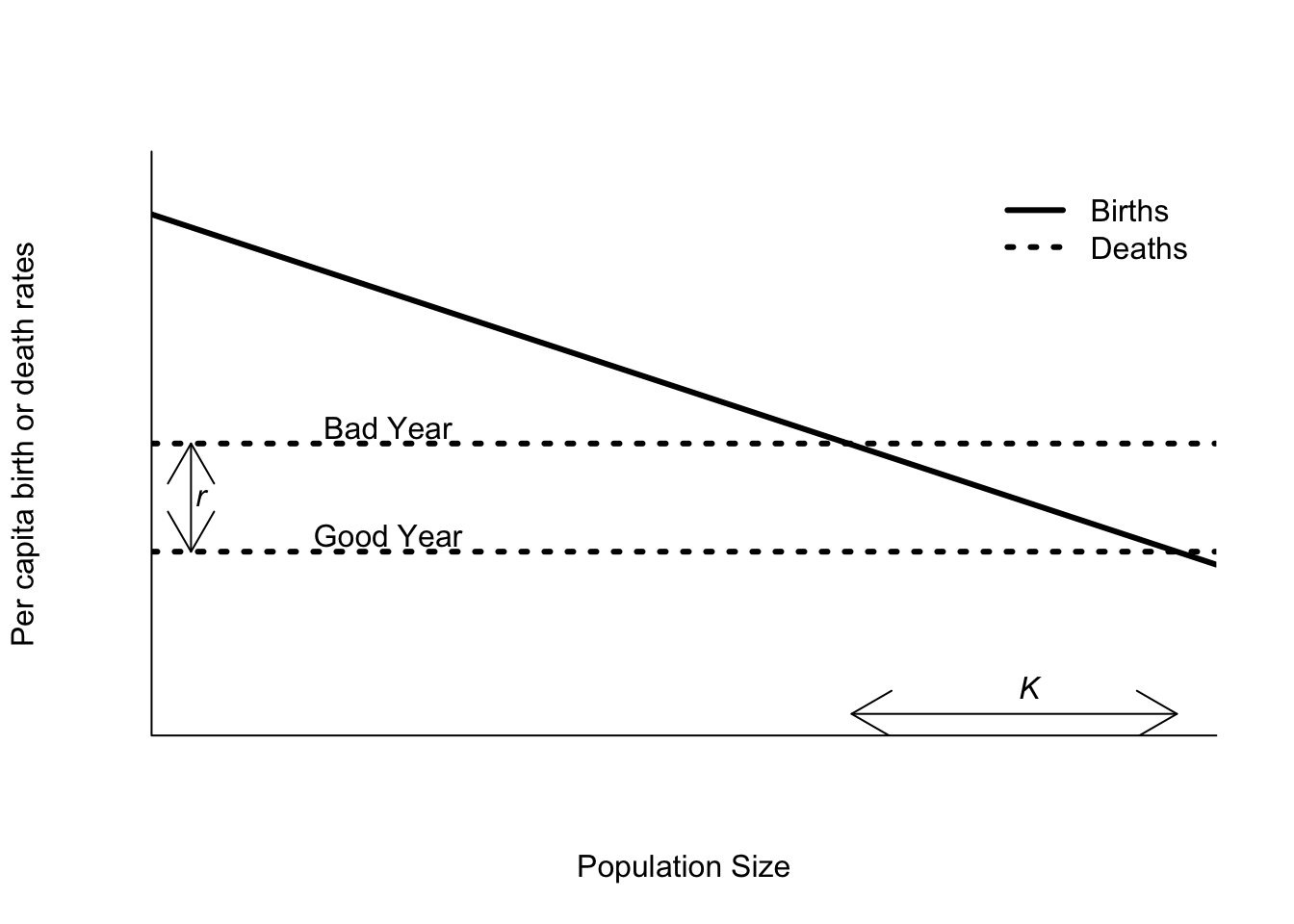
Figure 5.10: Per capita birth and death rates as functions of density as assumed by the logistic equation. The death rate can be either good or bad, depending on the year.
5.4 Trends over time
Stochastic variation in the vital rates of a population is one kind of change over time, but the sections above have assumed that the stochastic variation is stationary. A stationary distribution has statistical properties, ie. mean and variance, that are not changing with time. That is, even though the death rate in Figure 5.10 is different in each year, the mean death rate averaged across several years is not changing. What happens if the mean death rate does change with time? Figure 5.11 shows some of the possibilities. The most important feature is that the population size lags behind the changes in \(K\). This is easiest to see in the deterministic population model. \(K\) is decreasing linearly with time, but the population size does not decrease at the same rate initially. As the discrepancy between the population size and \(K\) gets larger, the negative pressure on population size increases until the point at which the population is decreasing just as fast as \(K\). After that point in time, both \(K\) and the deterministic population size decrease at the same rate; the lines on the graph are parallel. It turns out that the lag time between the start of the change in \(K\) and the point at which population size is decreasing equally quickly depends on the magnitude of the intrinsic growth rate \(r\). A population with large \(r\) will be able to track changes in \(K\) more closely, with a very short lag time. A population with small \(r\) will respond more slowly to changes in \(K\).
The other feature is that even small amounts of environmental stochasticity can create misleading trends over short time periods. For example, despite a decrease in carrying capacity, there are several periods where the population size subject to environmental stochasticity is relatively constant, or even increasing for a time. The trend in carrying capacity is influencing the average population size, but any particular time series will not necessarily track that average perfectly. The moral of the story is to be very careful about drawing grand conclusions from short time series.
Up until very recently it was common for earth scientists and ecologists to talk in terms of stationary systems – climate systems, ecosystems, and the like. However, given increasing awareness of large scale climate change, we should expect that systems are not stationary, and that trends in underlying vital rates should be the norm, rather than the exception. In addition, here in the Great Plains the landscape itself has not been stationary. Land use affects wildlife populations, and changing agricultural economics has led to large shifts in available habitats across the last half century or so. We have little information of sufficient extent in space and time to really understand what is going on.
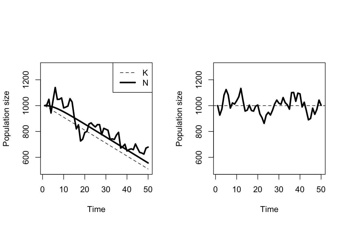
Figure 5.11: Ricker dynamics with and without a trend in carrying capacity. \(N_0 = K_0 = 1000, r=0.2\), and the rate of change in \(K\), \(k = - 10 / year\). The variance in population growth rates is \(\sigma^2 = 0.0025\). The left hand panel shows both deterministic and stochastic population growth.
5.5 Glossary
- Scramble competition all individuals in the population have equal access to resources.
- Regulated population a population that neither grows nor decays without limits.