Chapter 4 Exponential growth and decay
I want to revisit the fundamental law, and consider what happens when the rate constants are fixed. That is, the per capita rates of births, deaths, immigration and emigration are not changing with time.
\[\begin{equation} N' = bN - dN + i - e \tag{4.1} \end{equation}\]
4.1 Deaths
Of all the biological processes in the fundamental equation, the simplest one to get a handle on is \(D\), the number of deaths in a period of time. A great deal of fisheries and wildlife management involves directly manipulating \(D\) through harvest or culling, or indirectly manipulating \(D\) through habitat management.
Consider the problem of stocking a lake with walleye fingerlings. From past research at this lake, we know that the instantaneous mortality rate is \(d = 0.01 week^{-1}\). If a hatchery manager wants to stock 10,000 fingerlings, how many will survive one year? We have three pieces of information – the rate of mortality, the initial number of fish, and the period of time. In continuous time, assuming that there are no births, emigration or immigration
\[\begin{equation*} N' = - dN \end{equation*}\]
This is an equation for the rate of change in a variable where the variable itself (\(N\)) is multiplied by a constant. This is the equation for exponential decay. The solution to that equation is
\[\begin{equation} N_t = N_0 e^{-dt} \tag{4.2} \end{equation}\]
We can substitute in the values for our problem, where N0 = 10000 and t = 52 weeks, which gives us
\[\begin{equation*} N_{52} = 10000 e^{-(0.01)(52)} = 5945 fingerlings \end{equation*}\]
In nature, the result will almost certainly not be exactly 5945 fingerlings. We do not know \(d\) exactly, \(d\) might not be constant over the course of the year, and indeed, the process of mortality itself is not deterministic. We cannot know exactly how many fingerlings will encounter a channel catfish during the year; only that some will with catastrophic results for the fingerlings! The number 5945 is an expected value, in the sense of Chapter 3.
Instead of an instantaneous mortality rate, we might have a discrete time rate estimated from a mark-recapture program. In that case we would have a per capita mortality rate \(d_{\Delta t}=e^{-d \Delta t}\) Note that the discrete time rate depends on the interval over which it is estimated.
4.2 Births
The second term in the fundamental equation that we must have is the number of births in a single unit of time, \(B\). There is little that can be done to manage \(B\) directly; most wildlife management efforts can at best manipulate \(B\) indirectly by altering the habitat. There are instances where preventing births through contraception is a useful management strategy for over abundant species, but it is often more expensive than manipulating \(D\).
In the continuous time form, the rate of change in N from births is
\[\begin{equation*} N' = bN \end{equation*}\]
where b is the per capita rate of births per unit time. The population size after some interval of time \(t\), \(N_t\) will be given by
\[\begin{equation} N_t = N_0 e^{bt} \tag{4.3} \end{equation}\]
There are not very many species where births occur continuously (put in a box describing one of each type). Equation (4.3) is an approximation of what usually occurs with wildlife species, especially wildlife in temperate and polar systems. There are many circumstances in which this approximation is acceptable, but we must never forget that it is an approximation, not the objective reality. In Chapter 7 we will examine alternative approximations to the birth process that more closely match the biological reality.
4.3 Turchin’s law of population inertia
With births and deaths, we can proceed to construct the simplest possible model of population dynamics. In order to do so we must make an assumption about the remaining two pieces of the fundamental equation, \(I\) and \(E\), the number of individuals moving into and out of the population. We have a couple of choices here, but let us start with the simplest assumption: \(I = E = 0\). That is, we will assume that no individuals move into or out of the population. The population is closed to emigration and immigration. With this assumption, the fundamental equation in continuous time reduces to
\[\begin{equation} N' = bN - dN =(b-d)N = rN \tag{4.4} \end{equation}\]
where we’ve defined a new constant \(r\), the difference between the per capita birth and death rates. This constant \(r\) is so important in population dynamics that it has a special name – the intrinsic rate of population growth. Notice that equation (4.4) looks a lot like equation (4.2) and (4.3). It is the equation for exponential growth or decay, and we know the solution for that:
\[\begin{equation} N_t = N_0 e^{rt} \tag{4.5} \end{equation}\]
This is the equation for exponential population growth, and it is the simplest possible population model. When \(r > 0\), the population will increase, and when \(r < 0\) the population will decrease (Figure 4.1). Looking back at eq. (4.4), we can see that \(r > 0\) when the per capita birth rate is greater than the per capita death rate. That makes sense – in order for the population to increase the number of births must exceed the number of deaths. Conversely, \(r < 0\) when the per capita birth rate is less than the per capita death rate. The most important thing to recognize here is that the difference between a population growing or decaying is determined by the relative magnitudes of b and d. Measuring either one alone does not tell us whether the population will increase or decrease. What happens if \(r\) is exactly equal to zero? The population will neither increase nor decrease, but remain at exactly the same level.
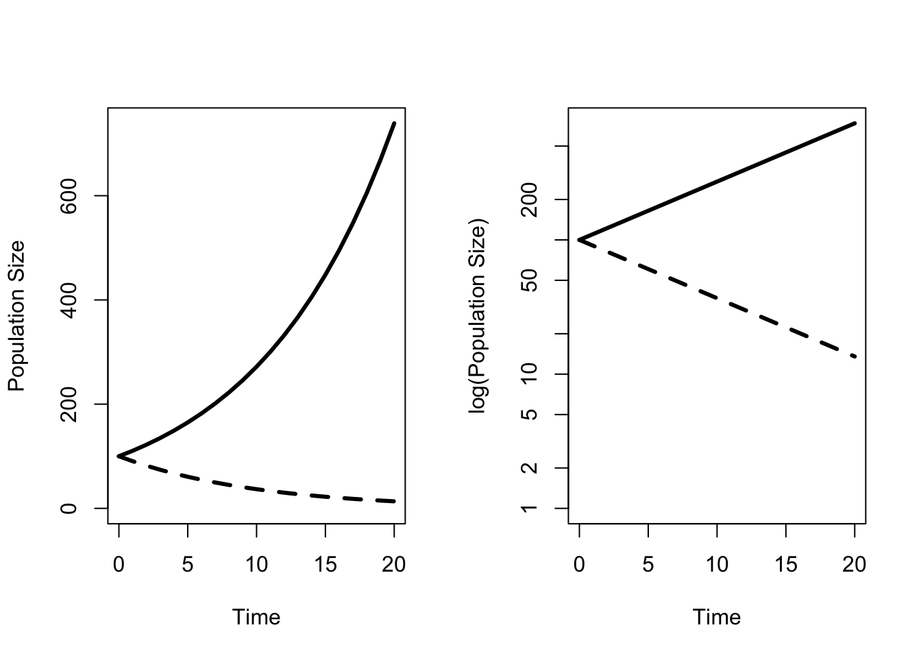
Figure 4.1: Population growth over time r is greater than or less than zero. The right hand panel shows the same curves on a log scale.
Turchin’s law of population inertia states: in the absence of other forces, a population will continue to grow (or decline) exponentially (Turchin 2003). Equation (4.5) tells us the rate at which the population will grow or decline. The important part of the law is the first phrase, “in the absence of other forces”. In particular, the birth and death rates are independent of the population size (Figure 4.2).
That is, assuming that the per capita birth and death rates remain constant, unaffected by other processes, then the law of population inertia holds. Much of the remainder of this book focuses on determining when the law of population inertia does not hold.
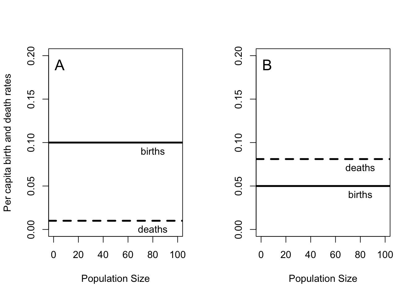
Figure 4.2: Per capita birth and death rates are independent of population size in exponential growth (A) or decay (B).
There is one additional property of the exponential model of population dynamics that makes it useful as a touchstone for analyzing changes in numbers. If we take the logarithm of both sides of Equation (4.5), we obtain
\[\begin{equation*} ln(N_t) = ln(N_0) + rt \end{equation*}\]
which has the same form as the equation of a straight line. The y-intercept of the graph is the logarithm of the population size when \(t=0\). Plotting the logarithm of \(N_t\) against time will then have a straight line with a slope of \(r\). This is a very easy way to check if a particular time series is well approximated by the exponential population model.
4.4 Estimating \(r\)
If this constant \(r\) is so important, how do we figure out what value to use? Later we will build up an estimate of \(r\) from detailed life history information. It can also be done in a “back of the envelope” way as long as we have two estimates of population size at different times. We start with equation (4.5), and rearrange it to solve for \(r\)
\[\begin{equation} \begin{split} \frac{N_t}{N_0} & = e^{rt} \\ ln\left(\frac{N_t}{N_0}\right) & = rt \\ r & = ln\left(\frac{N_t}{N_0}\right) / t \end{split} \end{equation}\]
So our first estimate of \(r\) is the log of the ratio of population estimates, divided by the number of time periods between the two estimates. This estimate assumes that the law of population inertia held during the intervening \(t\) time periods. As an example, let us carry out these calculations for the herd of Muskox (Ovibus moschatus) on Nunivak Island, Alaska. Muskox were extirpated from the Arctic slope of Alaska in the late 19th century, and efforts to reintroduce them from populations in Greenland began in the 1930’s. In 1947 David Spencer of the Bureau of Sport Fisheries and Wildlife in Alaska began an annual survey of the Nunivak Island population (Spencer and Lensink 1970). He recorded a total of 49 animals in 1947, and in 1965 he counted 514 animals total. Assuming that the law of population inertia held during those 18 years, we find
\[\begin{equation} r = ln\left(\frac{N_t}{N_0}\right) / t = ln\left(\frac{514}{49}\right) / 18 = \frac{ln(10.49)}{18} = 0.13 \, years^{-1} \end{equation}\]
How should we interpret that estimate? The change in a population over 1 year is \(Ne^r\), so the factor \(e^r\) is the percentage change in population size. In this case, \(e^r = 1.138\), or about a 14 % change per year. A useful approximation to remember is that when \(r\) is close to 1, then \(e^{r} \approx 1+r\), so you can think of \(r\) as a percentage change in population size per year as long as it isn’t too large. In the musk-ox case the error in this approximation is 1 percentage point.
With this estimate of \(r\) in hand, there are several things we can do. For example, what if we want to predict the number of animals on the island after another 3 years, assuming population growth holds at the same rate?
\[\begin{equation} N_3 = 514 e^{(0.13)(3)} = 514(1.48) = 759\,muskox \end{equation}\]
This is quite useful as a benchmark for management. If we go back in 3 years and there are a lot fewer, or a lot more muskox than we expected, then we would have to conclude that “all other forces” were not in fact zero, and that would start us on a useful search for what might have changed. In fact, in 1968 there were 714 animals. Is that a lot fewer than expected? In order to answer that question, we need to address an important issue – indeterminism – which we will begin in the next chapter.
Another easy calculation to do is finding the doubling time for a population. This is the number of years for the population to double in size. The key here is to recognize that a population has doubled when \(N_t = 2N_0\). We substitute \(2N_0\) into eq. (4.5) and solve for \(t\)
\[\begin{equation} \begin{split} \frac{2N_0}{N_0} & = e^{rt} \\ ln\left(2\right) & = rt \\ t & = \frac{ln\left(2\right)}{r}\,. \end{split} \tag{4.6} \end{equation}\]
For the musk ox we get \(t = ln(2)/0.13 = 5.3 \, years\) for the population to double in size. This calculation is very handy for guiding management expectations. If we desire a population to be 10% larger, we can calculate how many years that will take by replacing the constant 2 in eq. (4.6) with 1.1.
4.5 Glossary
- Instantaneous mortality rate the rate at which mortality events occur when the interval of time is allowed to shrink towards zero.
- Deterministic processes have only a single outcome given complete knowledge of the state of the system.
- Expected value of a random variable is the mean value, or the 1st moment of the distribution.
4.6 Exercises
An index of the Bald Eagle population in Illinois (Havera and Kruse 1988) grew from 188 individuals in 1970 to 569 individuals in 1987. Assuming a closed population with constant birth and death rates through this period, what was the annual population growth rate?
For the same population of Bald Eagles in Illinois, how many eagles would you expect in 1984?
If the actual population count in 1984 was 930, what could you conclude about this population?
In how many years would you expect the Bald Eagle population to double in size after 1987?
Wildlife managers at an east coast wildlife refuge want their population of Piping Plovers to increase by 20% in 5 years. Their estimated value of \(r = 0.01\) without changing any management strategies. Can they achieve their objective? What value of \(r\) would allow them to achieve their objective?
References
Turchin, Peter. 2003. Complex Population Dynamics: A Theoretical/Empirical Synthesis. Vol. 35. Princeton University Press.
Spencer, David L, and Calvin J Lensink. 1970. “The Muskox of Nunivak Island, Alaska.” The Journal of Wildlife Management. JSTOR, 1–15.
Havera, Stephen P, and Glen W Kruse. 1988. “Distribution and Abundance of Winter Populations of Bald Eagles in Illinois.” Champaign, Ill.: Illinois Natural History Survey.