Chapter 6 Harvesting and Control

Up to this point, I was content to let wildlife populations be. Now I want to mess around with them. In a closed population there are two options: alter per capita birth rates or per capita death rates. Both types of manipulation will result in changes to population size, which is often the objective of management. But some manipulations of death rates have a side effect of producing a flow of dead animals, ie. a harvest. This flow of dead animals can also be an objective of management if the animals have value after death. Value can arise from many things, including furs, meat, and trophies. Managers have to make decisions about whether, and how, to regulate harvest of wildlife populations. The same models of populations that help with harvest regulation can be used to make decisions about control of nuisance populations. Throughout this chapter I will talk about harvest regulation, but control of wildlife populations is just harvest with a different objective.

Eurasian Lynx in Norway

Everything is better with an example, and there is a great deal of information on the management of Eurasian Lynx (Lynx lynx) in Norway (Linnell et al. 2010). Lynx were widespread throughout Norway at the beginning of the 19^th century. As human populations grew, so did negative interactions with lynx. In 1846 the Norwegian government issued a bounty on lynx – essentially paying for dead lynx – which remained in place until 1980. Throughout that period the allowed methods for taking lynx were reduced, and populations recovered somewhat from their lowest levels in the 1940’s. In 1976 lynx were restricted to two small remnant populations, and were listed on the CITES Appendix II. After the bounty was removed, hunting was still allowed. The season was restricted starting in 1982, but there were no restrictions on the number of lynx taken. Lynx populations began to recover according to records of the number of lynx harvested. Managers regarded these records as relatively accurate because there was little incentive to poach, given the lack of restriction on harvest. Throughout the 1980s and early 1990’s the number of lynx taken annually was less than 50.

In 1992 public outcry over the harvest of a mother and both of her kittens by a hunter led to a temporary cessation of all hunting. Finally, in 1994 a regulated harvest with a restricted season and a nationwide quota of 47 animals was allowed. In addition, a program that compensated livestock owners for losses to lynx and other large carnivores was put in place. Population size of lynx has been estimated using consistent methods since 1996 (Figure 6.1). Quotas were greater than 25 to 30% of the estimated population size, and populations declined steadily until 2004. Since 2004 quotas have been kept less than 20% of the estimated population size. Annual variation in the number compensation payouts have mirrored variation in estimated population size.

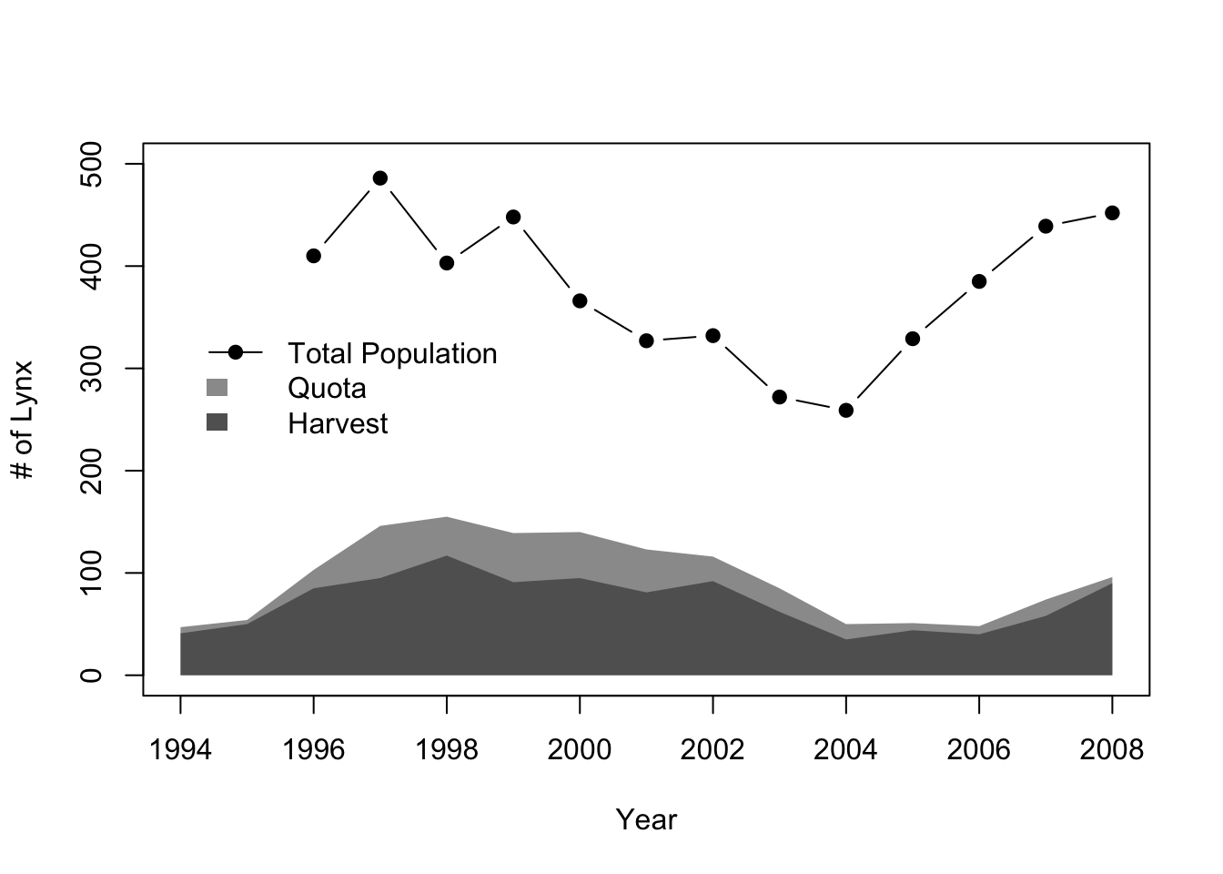
Figure 6.1: Estimated number of lynx in Norway, the annual hunting quota, and the # harvested since 1994.

6.1 Compensatory and Additive Mortality

A common paradigm in wildlife science is the distinction between compensatory and additive mortality. This distinction is usually made when referring to anthropogenic, or human-caused, mortality such as harvest. If anthropogenic mortality is additive, it means that the total death rate is the sum of anthropogenic mortality and natural mortality. If anthropogenic mortality is compensatory, it means that natural mortality is reduced such that the total death rate is unchanged. Clearly compensatory mortality is very useful, even essential, if the objective is to sustainably harvest a population. A typical depiction of the distinction is shown in Figure 6.2. As anthropogenic mortality increases the probability of survival decreases in the additive case. Any degree of extra mortality reduces survival probability. In contrast, as anthropogenic mortality is increased in the compensatory case, the probability of survival does not decrease, at least initially. Eventually the extra mortality becomes too great, and the survival probability begins to decrease. The rate of decrease is not specified, but it will not lead to survival probabilities that are less than those under the additive case. I call this the “standard model” of wildlife harvest. Typically the assertion is that harvest rates up to the point of compensation are sustainable. The distinction between compensatory and additive mortality was a central part of debates over waterfowl harvest in North America throughout the 1970’s, 1980’s and beyond.

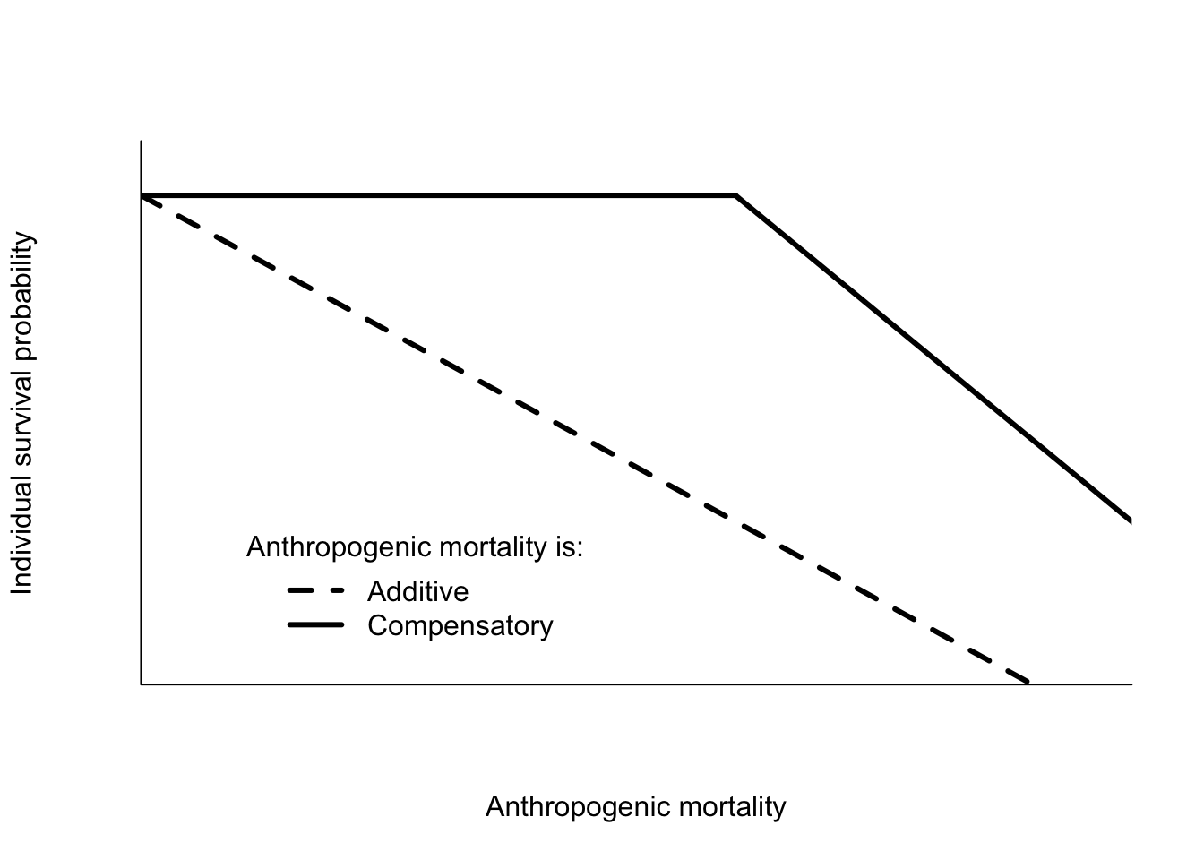
Figure 6.2: Hypothetical survival probabilities for individuals under additive and compensatory mortality.

The mechanism that creates compensatory mortality is a density dependent change in natural mortality rates, like that assumed under the logistic population model. Anthropogenic mortality reduces the population size, and the remaining individuals experience lower natural mortality. However, the standard model is misleading for at least two reasons. First, as shown in the previous chapter, populations that are regulated by density dependence may not have changes in mortality. Increasing density could reduce birth rates instead of increasing death rates. Or both birth rates and death rates could change. Second, population size must decrease in order for compensatory decreases in death rates to occur. The standard model does not show this effect because it plots survival against harvest rate, not population size (Figure 6.2).

6.2 A Better Model For Harvesting Wildlife

We can obtain a much richer understanding of what is going on with wildlife populations under harvest, or indeed, under any kind of increased anthropogenic mortality by using the graphical techniques from Chapter 5. I will start with a plot of the population growth rate versus the population size (Figure 6.3). Ignoring environmental and demographic stochasticity, you know that the population will reach a stable equilibrium at \(K\). At that point, the population growth rate is zero. Now imagine that you harvest a fixed proportion of the population, \(h\). This is a straight line on our graph with a slope of \(h\), because the amount harvested (and hence the change in \(N\)) increases with population size. This creates a new equilibrium point where the population growth rate is equal to the harvest rate, and the total rate of change is again equal to zero. The most important point to recognize is that this new equilibrium point is \(<K\). Harvesting reduces population size. Always. A decrease in population size under harvest does not necessarily mean the harvest is unsustainable. For a logistic population, a fixed proportional harvest always has a positive equilibrium population unless \(h > r\). A harvest that large has no positive intersection with the population growth rate curve, and thus the only equilibrium point is \(N=0\).

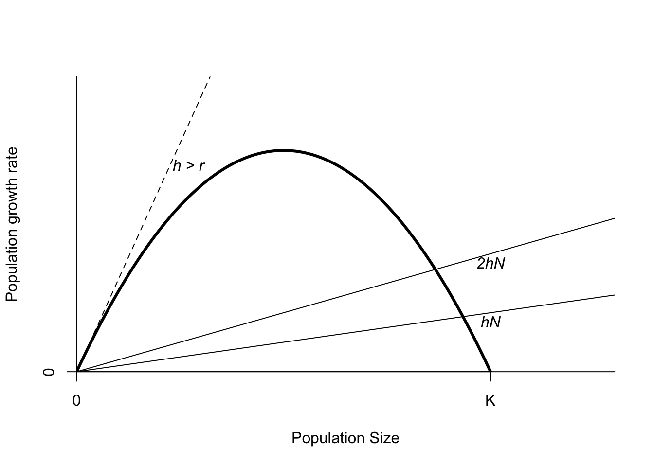
Figure 6.3: Population growth as a function of population size. The thin lines show the effects of a fixed proportion of harvest.

As the per capita harvest rate h increases, the population decreases. What happens to the number of animals actually harvested? A little bit of algebra will get us the answer. We start with the discrete Logistic model with an additional term for the harvest rate, and then do some algebra to figure out how many animals are harvested at the level \(h\). The math is identical for a continuous time model, but you can use this equation in R. This equilibrium harvest is \(H^*\).

\[\begin{equation} \begin{split} N_{t+1} & = N_t+N_t r\left(1-\frac{N_t}{K}\right)-hN_t \\ N^* & = K^*\left(1-\frac{h}{r}\right) \\ H^* & = hN^* = hK\left(1-\frac{h}{r}\right) \end{split} \end{equation}\]

These equations are shown in Figure 6.4. There are two important features to note. First, as harvest rate increases, the heavy dashed line rotates up and to the left, and the equilibrium population size decreases. Second, as harvest rates increase, the total harvest first increases, reaches a maximum value at \(r/2\), and then decreases. This means that for any particular total harvest \(H\), there are two different harvest rates that will achieve it. The higher harvest rate corresponds to an equilibrium population size that is less than half the carrying capacity. Although this equilibrium is stable, populations in this state are described as “overexploited”, because there is a lower harvest rate that will produce the same total yield at a higher equilibrium population size. In the overexploited state, increased harvest leads to decreased yield. The harvest rate that generates the maximum yield, \(r/2\) is also called the Maximum Sustainable Yield, or MSY. The total amount harvested at that point is \(rK/4\).

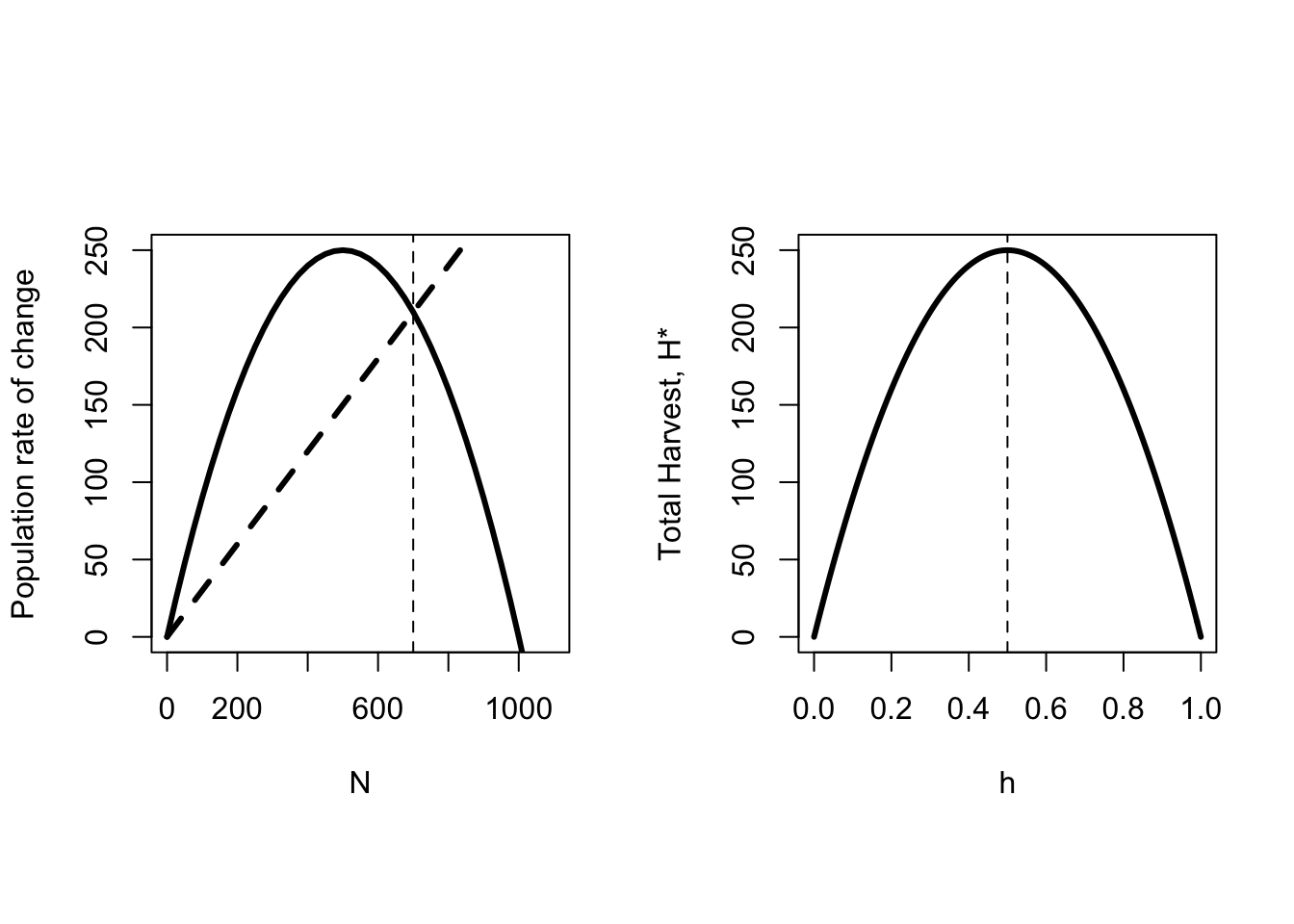
Figure 6.4: In the left panel the population rate of change (solid line) for the discrete Logistic model with a fixed proportional harvest (dashed heavy line) is plotted against population size. The parameters are \(r=1\), \(h=0.3\) and \(K=1000\). The vertical dashed line is the population size under harvesting pressure. In the right panel the total harvest \(H^*\) is plotted against the per capita harvest rate. The vertical line shows the maximum harvest occurs at \(r/2\).

Epitaph for MSY

Peter Larkin wrote the following poem in his 1977 paper outlining why aiming for MSY was a bad way to manage a commercial fishery.

Here lies the concept, MSY.
It advocated yields too high,
And didn’t spell out how to slice the pie.
We bury it with the best of wishes,
Especially on behalf of fishes.
We don’t know yet what will take it’s place,
but we hope it’s as good for the human race.

6.2.1 Fixed quota harvesting

What are some other ways we could harvest a wildlife population? It is quite typical for recreational harvests to be regulated by controlling the total number of animals harvested. I call this a fixed quota harvest strategy. If the quota is always filled (a big assumption), then the per capita harvest rate is \(\frac{Q}{N}\), and the population harvest rate is a flat line (Figure 6.5). As before, there is an equilibrium point \(K'\) with a positive amount of harvest that is just a bit less than \(K\). This equilibrium point is stable. When the population size is greater than \(K'\) harvest rate exceeds the population growth rate, and the population will decrease back toward \(K'\). If the population size is lower than \(K'\), then the population growth rate is greater than the harvest rate, and the population will grow.

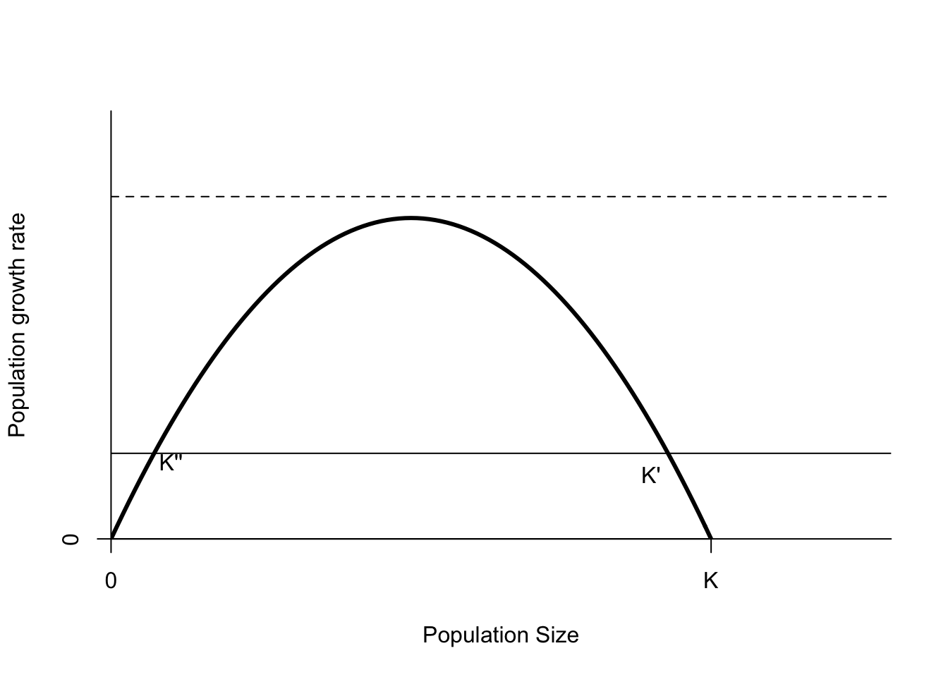
Figure 6.5: Population growth as a function of population size. The thin line shows the effects of a fixed quota \(Q=0.2K\). The thin dashed line is a fixed quota of \(Q=0.9K\). The parameters of this curve are \(r=3\) and \(K=1\).

What about the point \(K''\)? It is an equilibrium point because the harvest rate and population growth rates are equal. However, \(K''\) is not stable. If the population is reduced below \(K''\), the harvest rate exceeds the population growth rate, and the population will decrease. The next equilibrium point is \(N=0\), which in this situation is a stable point. If the population size falls below \(K''\), and harvest is maintained at \(Q\), harvesting will drive the population extinct.

The other way to drive a population extinct with fixed quota harvesting is to set the quota \(Q > rK/4\). Recall that the peak of the population growth rate curve in Figure 6.5 is \(rK/4\). This quota corresponds to a flat line that is higher than the parabola representing the population growth rate. In other words the harvest is greater than the population growth rate for all population sizes.

Harvesting a fixed proportion is considered safer than a fixed quota, because a fixed proportion doesn’t lead to the formation of an unstable limit, unless the harvest rate is very high (\(h > r\)). As the population size decreases, so does the harvest. However, the difficulty with a proportional harvest is that it requires an accurate estimate of population size. If your estimate is high, \(\hat{N}>N\), then actual proportional harvest is higher than assumed. That means that the equilibrium \(K'\) is closer to the peak of the population growth rate curve, and \(h\) is closer to the limit \(r\) that will cause the population to go extinct.

6.2.2 Fixed Effort harvest strategy

It is worth asking if there is a way to get a “safe” harvest without knowing the population size exactly. Instead of regulating the harvest directly, it is also possible to regulate the effort that harvesters put in. The assumption is that harvest rate increases with the amount of effort. This is often done by limiting the duration of the period harvesters are allowed to operate, or by limiting the gear that they can use. By restricting effort, the harvest rate adjusts naturally to the abundance of the population without knowing the population size.

The simplest model of effort is \(h = qE\), where \(E\) is measured in units of effort (days, fishing lines, etc.) and \(q\) is a “catchability coefficient” which describes how harvest rate changes with effort. If effort is fixed over time, and \(q\) remains constant this model will have the same dynamics as a fixed proportional harvest, but does not rely on an estimate of population size.

Effort can change in different ways. Many commercial fisheries have collapsed in part because of failures to account for “effort creep”. For example, in the 1950’s a prawn fishery developed in the Gulf of Carpenteria on Australia’s northern coast. A typical boat was less than 50’ long, and could tow a trawl net that covered 30-40’ of bottom. The fishery was regulated by the number of days and the number of licenses (units of boat-days). By the time I worked on the Northern Prawn Fishery in 2002, a typical prawn trawler was > 200’ long and capable of towing 4 trawls simultaneously! Add to that GPS locator capability, sonar depth sounders, and you have a machine vastly more efficient at harvesting than the boats of the mid twentieth century. A boat-day in 2001 was not the same as a boat-day in 1955. Effort creep leads to an increase in the catchability coefficient \(q\).

Another example of the effect of controlling effort comes from Oregon’s sport harvest of cougars (Puma concolor). The history of Oregon’s cougars is similar to Norway’s Eurasion lynx; near eradication followed by a steady recovery. A regulated sport harvest has been in place since 1970 (Figure 6.6). For the most part, the harvest has been managed as a fixed quota which has rarely been filled. The biggest change in effort occurred in 1994 when the use of hounds to track and tree cougars was outlawed by a Ballot proposition (Period D in Figure 6.6). The rate of successful harvests plummeted. In response, the Fish and Game commission added mountain lions to a multi-species license package, which meant that many more hunters could opportunistically take lions even if they were not searching for them specifically. Eliminating hounds reduced the effectiveness of hunters (reduced \(q\)), so to maintain harvest rates the number of hunters was increased (increase \(E\)).

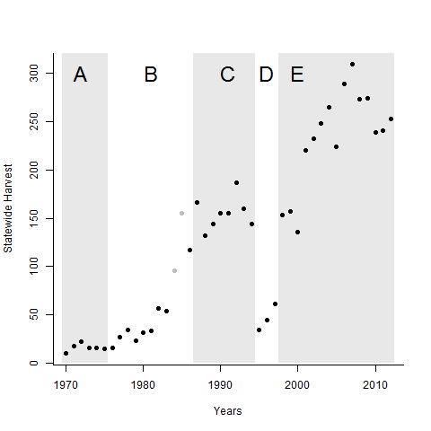
Figure 6.6: Total statewide cougar harvest by hunters from 1970 to 2012, Oregon, USA. Grey rectangles indicate periods with major regulatory changes related to distinct harvest regulations. Points shaded grey are partial counts, as no records were kept for portions of the state. A: unknown regulations. B: increased quotas. C: All harvested animals submitted for aging, hounds allowed, species specific license. D: Hounds outlawed by ballot proposition. E: Addition of mountain lions to the sport-pac multispecies license. Adapted from Tyre et al. unpublished ms.

6.2.3 Revisiting Eurasian Lynx

So how is the Eurasian lynx harvest managed? It seems to be a bit of a hybrid. There is a quota, but it is adjusted continuously as the harvest size changes as if attempting to maintain a fixed proportion. It is not clear what the target proportion was, because there is no fixed proportion. There is an additional wrinkle too — the quota is not filled each year. That is, there are some hunting opportunities that are not taken. This could arise either because of a lack of hunters, a lack of animals, or both. Variation in the degree to which harvest goals are achieved could be treated as another source of stochasticity in the population dynamics. One term used for this is implementation uncertainty (Bischof et al. 2012).

This sort of variability is quite common in recreational harvest systems, and makes understanding them much more difficult than commercial harvest systems. In a commercial harvest you can rely on harvesters to aggressively maximize their economic benefit. The benefit to a recreational harvester for hunting is more complex. In addition to the obvious food, fur, or trophy, recreational harvesters just like to be outside. As a result, simple things like a particularly cold day or the scheduling of a popular football game can have an effect on the level of harvest. You might think the football game is a far-fetched example, but the effect has been noticed by Nebraska Game and Parks staff at deer check stations!

Prior to 1994 the lynx harvest was averaging less than 50 individuals per year, even though it was unregulated. In 1996 and 1997 the quota was raised to more than double this level, and harvests also increased substantially. The population began to decline, but if our model is correct, this would be expected. Even if the quota had not been reduced in response to the decline, I would have expected the population size to level out at a new equilibrium. However, the quota was reduced steadily, until 2004 when it was reduced by a large amount. Subsequently to that the population began to increase again! I can only imagine the degree of angst and political wrangling that goes into these decisions.

6.2.4 Revisiting Additivity

It is important to recast the additive mortality paradigm into our improved model. The charge of additive mortality is frequently used by political opponents of hunting to argue for reduced or eliminated harvest. The only kind of population that will not experience a compensatory increase in population growth rate is a population that is growing exponentially. In an exponentially growing population both the birth rates and the death rates are independent of population size (Figure 6.7). If the harvest rate is less than \(r\), then the population continues to grow exponentially, albeit at a slower rate. If the harvest rate is greater than \(r\), the population will decline exponentially. The only harvest rate that will keep the population from either increasing or decreasing is exactly \(r\). In the face of environmental stochasticity, estimation error and implementation uncertainty, this is impossible to achieve.

That does not mean that harvest mortality is never additive. The additional wrinkle to keep in mind is that it is possible for the relationship between vital rates and population size to change over time. In particular, animals in strongly seasonal evnironments or that migrate long distances may experience very different environments at different stages of the year. Mule deer (Odoceilus hemionus) in Colorado show density dependent decreases in survival during severe winters, but not during mild winters (Bartmann, White, and Carpenter 1992, @unsworthetal1999). Thus, the demographic response to a fall harvest will be different in years with mild vs. severe winters. In a year with a mild winter the fall harvest mortality will be more additive, with no compensatory decrease in mortality of individuals that survive harvest.

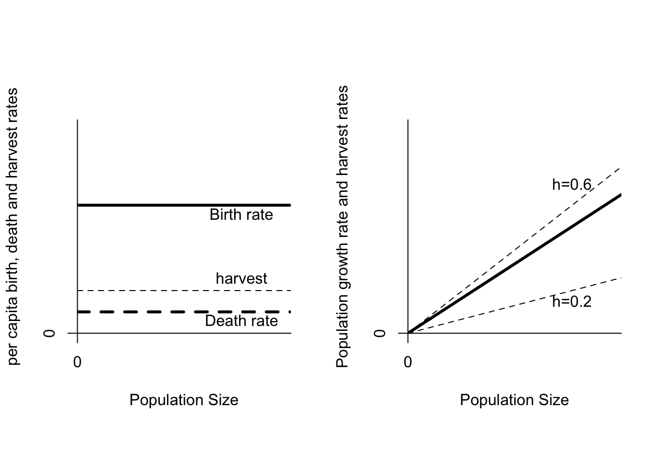
Figure 6.7: On the left are per capita birth (b=0.6), death (d=0.1) and harvest rates (h=0.2). On the right is population growth as a function of population size. The thin lines show a proportional harvest at h = 0.2 or h=0.6.

6.3 What about control?

Control is usually suggested when stakeholders are experiencing negative impacts from the species. Biologically, there is no difference between harvesting a population and culling a population to reduce damage. The only difference is the objective. Typically the objective of harvesting is to allow the total harvest to be as large as possible without driving the population extinct. In contrast, the objective in control situations is usually to reduce the population size as efficiently as possible. If the relationship between population size and impact is linear, then it is sufficient to express the objective of control in terms of population size.

Although negative impacts usually decrease utility as population size increases, this decrease may not be linear. In that case it is important to express the objective directly in terms of the reduction in damage. This will result in control programs that are more effective (in the sense of reaching acceptable damage levels), and more efficient (in the sense of using the smallest amount of effort needed). Some of these possibilities are shown in Figure 6.8. Assuming that the relationship is proportional might lead to the population target shown by the dot. If the actual relationship is given by curve A, then this population level target will not reduce the damage to socially acceptable levels. In contrast, if the relationship between population size and damage is given by curve B, then the population objective will be inefficient, reducing the population much more than is needed to achieve a level of social acceptance.

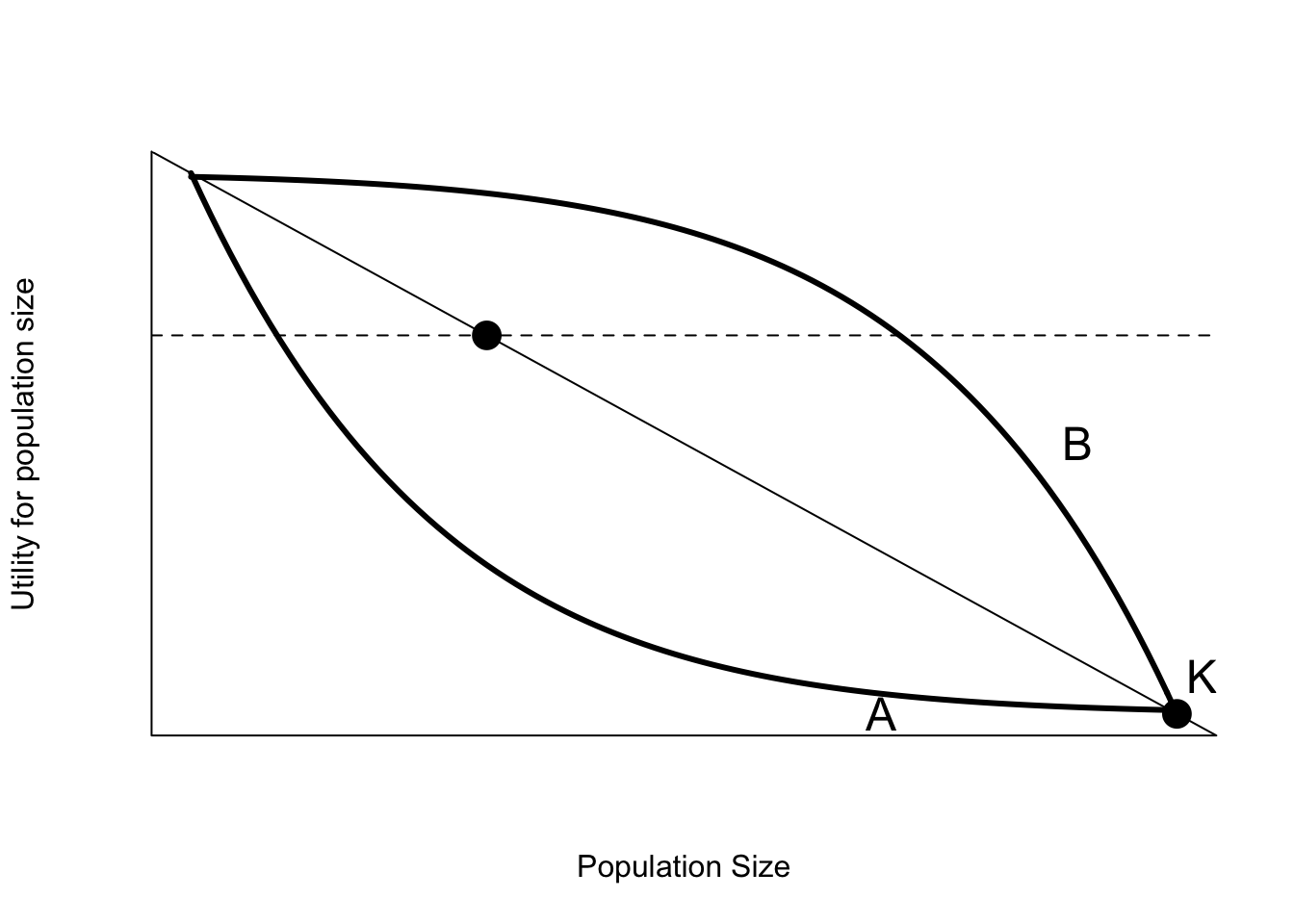
Figure 6.8: Some possible non-linear relationships between utility and population size. The dot labelled K is the current population size and level of damage. The thin solid line represents the assumption that damage is proportional to population size. The thin dashed line represents the socially acceptable level of damage. The dot represents a population level objective assuming that damage is proportional to population size, and the socially acceptable amount of damage is 30% of current levels.

The other advantage of expressing control objectives directly in terms of levels of impact is that it helps expand the range of possible alternatives. If the conversation focuses exclusively on population levels, culling tends to be the first and often only option considered. Thinking in terms of population dynamics broadly opens up additional options. For example, rather than increase direct mortality rates it is also possible to reduce birth rates by various means. That changes the shape of the population growth rate curve, and can reduce equilibrium abundance. Thinking directly about damage levels opens up even more opportunities. For example, sometimes it is possible to move a population around a landscape, so that they spend more time in areas where they cause less damage. This can work by a combination of attractants (e.g. feeding stations) and/or dispersants (e.g. bangers). A particularly interesting strategy for keeping birds off of runways is to use trained falcons to increase the perceived risk of foraging on the runway.

Joel Berger put forward the idea of a “landscape of fear” in his 2009 book “The better to eat you with: fear in the animal world” (Berger 2009). If animals are afraid of predators, they alter their behavior to reduce that fear. In Yellowstone National Park the reintroduction of wolves resulted in a change in behavior by elk herds to shift their foraging away from riparian areas favored by wolves. This had a beneficial side effect of reducing elk damage on fragile riparian vegetation. At the present time Rocky Mountain National Park is also experiencing high levels of vegetation damage by large populations of Elk. Rather than reducing elk populations by allowing hunting in the national park, perhaps another wolf introduction is warranted?

6.3.1 Predicting the response to management

Regardless of how the manipulation is achieved, it is necessary to predict how much effort is required to achieve the objective. The improved model of wildlife harvest can be used for predicting the effects of control efforts that increase death rates. If the goal is to eliminate the population, and a fixed quota \(Q\) can be taken, then we need to set the effort at a high enough level to exceed the Maximum Sustainable Yield (Figure 6.5) which is \(rK/4\). Levels of effort that lead to per capita harvest rates less than \(r/2\) will reduce the population, but not drive it extinct.

Specifying a particular quota in a control situation is usually unrealistic, because the effort required to reach the quota increases as population size decreases. In a commercial harvest situation effort will increase as population size decreases because that is how harvesters maximize profit. In a control situation someone or some agency must expend money to increase effort, and in practice that means there is an upper limit to effort. That in turn means that the “proportional harvest” model is more appropriate. In that case, driving a population extinct requires a per capita harvest rate \(h>r\), or double the fixed quota harvest rate!

Predicting the effect of a change in birth rates needs the underlying model of population regulation to be specified (see Chapter 5). If we do something that affects birth rates equally at all population sizes, then the per capita birth rate curve shifts downwards (Figure 6.9; green line). This reduces both \(r\) and \(K\) in the logistic equation, and leads to a smaller population size. It is also possible that some management actions affect individuals more in larger populations. For example, reducing the total amount of habitat will have this effect, leading to a steeper decline in the per capita birth rate with increasing population size (Figure 6.9; blue line). This reduces \(K\) but not \(r\).

Driving a population extinct by reducing birth rates requires enough effort that the entire per capita birth rate curve drops below the per capita death rate curve. Thus it is not necessary to reduce birth rates to zero, but rather get them lower than per capita death rates at all population sizes.

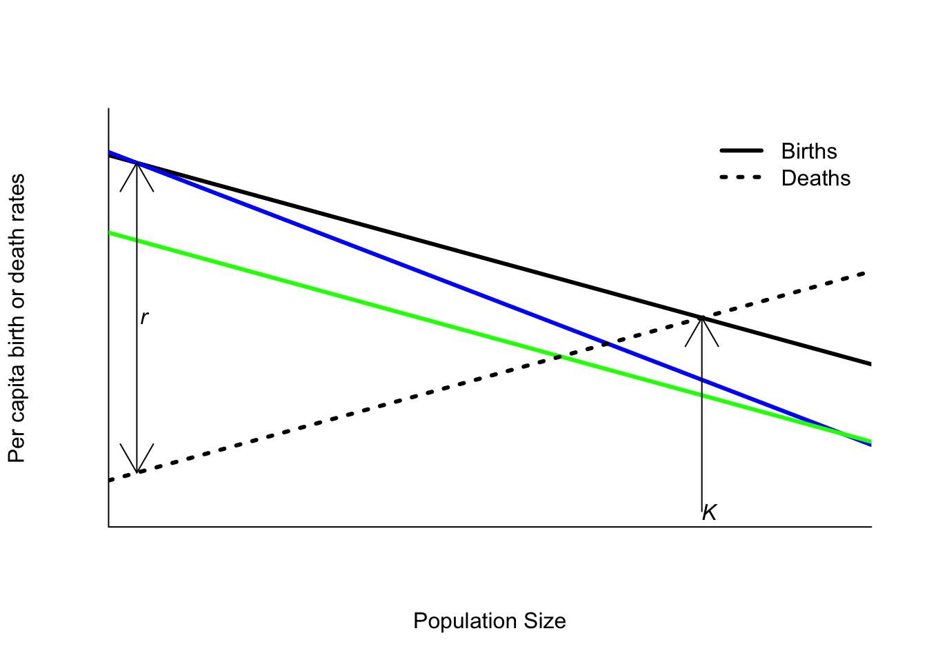
Figure 6.9: The effect of reducing per capita birth rates when a population grows according to the logistic equation. Blue: increasing effect of competition (e.g. reducing habitat, removing food). Green: decreasing reproduction at all densities (e.g. sterilizing individuals)

Imagine you have a population of Koala (Phascolarctos cinereus) growing according to the logistic model, and currently at the maximum carrying capacity \(K\) (Figure 6.10). This population is disease free, and unfortunately the Eucaplytus population that provides all their food cannot sustain this population level for very long. Eventually the koalas completely defoliate and kill their food source unless their populations are maintained below a critical threshold (vertical red line in Figure 6.9). We have to choose between 3 different levels of culling (fixed annual quotas), and a surgical sterilization program that reduces birth rates at all densities, and thus reduces both \(r\) and \(K\).

First, note that the only strategy that can reduce the Koala population below the critical threshold on its own is culling at level 3. Culling at level 1 or 2 reduces the population size somewhat, but these lead to stable equilibria above the critical threshold. The sterilization campaign reduces the population more, but still ends up at a stable population size above the critical threshold. The only stable point below the critical threshold is \(K'''\), which involves a combination of sterilization and culling at level 1.

Sterilization changes the population growth curve, but does not immediately reduce population size. It is also very expensive. It may be cheaper and quicker (safer for the trees!) to cull at level 3 until the population is below \(K'''\), then reduce culling and start sterilization.

If we could accurately count koalas, then a proportional harvest rate strategy that intersects the population growth curve to the left of the critical threshold would also yield a stable equilibrum. This point puts the population in the “overexploited” state. The risk is that having the harvest rate too high might put the population at risk of extinction. This risk is also present for the culling/sterilization strategy. Which strategy is “riskier” depends alot on the shape of those growth rate curves, how accurate the population estimates are, and how much environmental and demographic stochasticity is present in the population.

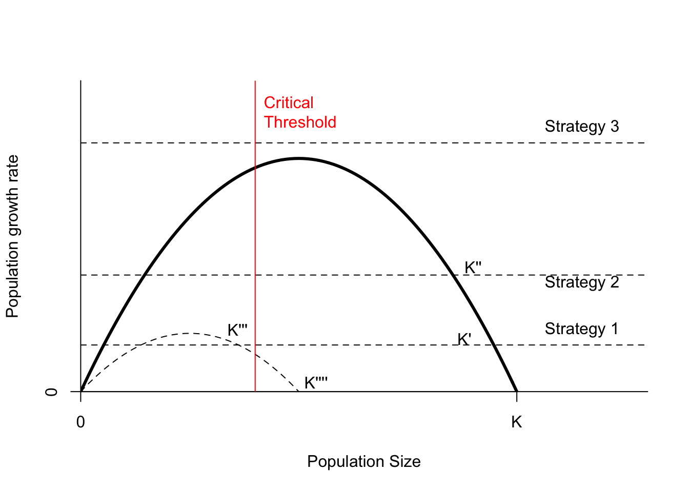
Figure 6.10: Population growth as a function of population size. Strategies 1, 2, and 3 represent different fixed quota culls. Strategy 4 represents surgical sterilization of half the population. The parameters of the solid curve are \(r=3\) and \(K=1\); the dashed curve (sterilization) is \(r=1.5\) and \(K = 0.5\). The dots mark unstable equilibria; stable equilibrium points are labelled \(K\).

Mid continental light geese

The mid-continental populations of light geese (Lesser Snow Goose and Ross’ Goose) cause extensive damage to salt marsh habitats in their sub-arctic and arctic breeding grounds. In 1997 the Arctic Goose Joint Venture (AGJV) issued a report detailing the extent of the damage along the south coast of Hudson’s Bay, and recommended efforts to dramatically increase harvest by recreational hunters to reduce the population and protect these habitats. Populations of light geese began to increase after food availability in their wintering habitats increased with changes in agricultural practices, improving overwintering survival. In addition, numbers of hunters declined steadily throughout the 2^nd half of the 20^th century, reducing harvest mortality. Increased survival leads to an increase in population size even if the population is regulated by density dependence in birth rates (see chapter 5).

The effect of increased goose foraging on fragile salt marsh habitats appeared to have a threshold response. Marsh vegetation could sustain low levels of foraging, but as foraging increased it reaches a point at which above-ground vegetation is completely removed. At that point, the feedback processes that keep soil salinity in check are removed, and soil salinity rises (Jefferies et al 2006). Marsh plants find it difficult or impossible to reestablish in high salinity soils, and the marsh remains as a mudflat even after goose foraging decreases. This is an interesting example because our utility, measured by the persistence of salt marsh vegetation, is high and relatively independent of goose populations until they reach high levels (Type B curve, Figure 6.8). However, once the threshold is passed, the utility curve will flip to a Type A curve, where utility is low until the population size is dramatically decreased!

So what happened with the light goose population? The primary recommendation from the AGJV report was to increase mortality on adult geese during the spring when it was thought that mortality would be additive in effect (see the standard model of wildlife harvest). The degree of political support garnered from both American and Canadian governments was tremendous, and resulted in changes to the Migratory Bird Treaty Act to allow extended hunting seasons. However, despite longer hunting seasons, no bag limits and dramatically reduced regulations on how hunters could approach light geese by states and provinces, populations have continued to increase. Although the changes in regulations increased harvest rates for some breeding colonies, the increase was only temporary. This suggests that harvest is limited by effort, primarily the number of hunters rather than time or their individual effectiveness. As a result, increasing populations lead to decreases in the per capita harvest rate of geese. In the most recent assessment (AGJV 2012) the growth rate of light goose populations appears to be decelerating towards an equilibrium as we would predict from the improved model. The real question to be answered now is whether we humans are satisfied with the amount and distribution of salt marsh habitats that will be present at this new equilibrium.

Living with large predators

In both Norway and Oregon there has been an increase in the number of lynx and cougars. Elsewhere in North America cougar and wolf populations have also increased. These large predators readily attack and eat livestock, and as populations increase, the number of complaints from livestock producers increases too. In Oregon, a complaint from a livestock producer usually results in the death of the cougar on a depredation permit.

At low populations cougars are restricted to areas of their preferred habitat in Oregon - undisturbed forested mountains. There are relatively few livestock in these areas. However as populations increase, young animals are increasingly forced out of preferred habitats into areas preferred for livestock production. This leads to an increase in complaints by producers. The utility curve from a producers perspective is probably sigmoid. At low population size producer utility is high, and it remains high until cougars are pushed out of wilderness areas. I suspect that once livestock predation begins to occur that a producer’s utility decreases very rapidly. Thus producers may want zero lions in their immediate vicinity, but be more tolerant of lions elsewhere.

It is instructive to think about the utility curves of other groups of stakeholders. Groups like the Mountain Lion Foundation heavily criticize sport harvest of cougars in North America and wish to see larger populations of cougars. The MLF utility curve is low or even zero at low populations of cougars, and presumably increases with increasing population size. There does not appear to be a population size for cougars above which the utility for groups like the MLF levels off, or if there is, it is well above the present abundance and distribution of mountain lions.

In recent decades a new group of stakeholders has emerged, urban dwellers whose homes begin to intersect expanding populations of cougars. David Baron documented this process along Colorado’s front range in his book “The beast in the garden” (Baron 2010). For people living in these areas it seems reasonable to think that their utility also increases with increasing populations of lions as for the MLF. However, it also seems likely that as populations get large enough that people feel pets, children, and themselves are at risk, that their utility begins to decrease.

The fact that different subsets of society have different utility functions for the population size of cougars in a region is what makes large predator management controversial. Regardless of what is done, there is someone whose utility would be improved by a different choice. If that someone has sufficient political clout with their state or federal representative they will be better able to improve the outcome for themselves. Rather than bemoan the fact that large predator management is political, wildlife biologists need to embrace that fact, and accept that what we personally want may not be what happens.

6.4 A “rule of thumb” for harvest and control

Managing wildlife populations is difficult even in the best of cases where managers devote substantial effort to data collection and analysis. Michael Runge and colleagues from the USGS developed a formula for determining “prescribed take level” for a species (Runge et al. 2009). The formula is derived from the logistic model of population growth, and is an extension of “Potential Biological Removal” formula written into the Marine Mammal Protection Act. Recall that the maximum sustainable yield for a population growing according to the logistic equation is

\[\begin{equation} MSY = \frac{r_{max}}{2}N^*. \end{equation}\]

Harvest, or take, less than MSY will be sustainable in the sense of having a positive equilibrium population size \(N^*\). Runge et al. introduced a new “management objective” variable \(F_0\) which ranges between 0 and 2. The prescribed take level in year \(t\) is then

\[\begin{equation} PTL_t = F_0 \frac{\tilde{r}_{max}}{2} \tilde{N}_t. \end{equation}\]

The \(\tilde{}\) over \(r\) and \(N\) are there to remind you that these quantities are not known exactly. A management objective \(F_0 = 0\) corresponds to no allowed take, and the population will eventually stabilize at \(K\). A value of \(F_0\) greater than 1 corresponds to an objective of driving a population close to zero. The advantage of specifying take in this manner is that we do not have to estimate \(K\). All we need to know is the current population size, and the species potential for population growth at low population sizes.

It is instructive to work backwards from harvest quotas set by management agencies (ie. PTL) using agency estimates of \(N_t\) and \(r_{max}\) to infer what sort of management objective is in place. Nebraska recently opened a mountain lion season for the Pine Ridge area in 2014. There were two short seasons, and no more than 2 males could be taken in each season. If a female was taken the entire hunting season would close. As it turned out, 3 lions (two males, one female) were harvested in total, out of an estimated population of 22. Ignoring uncertainty, and using \(r_{max} = 0.28\) from the literature, \(F_0 = 0.97\). This is approximately an MSY harvest, and the expectation is that the population will stabilize around half of the carrying capacity.

There are a few reasons to think this might be an optimistic view of the allowed harvest. First, this simple model ignores sex structure of the population. A maximum of 4 males out of the male portion of the population alone is a harvest that will depress male population size much more than MSY levels. Second, the estimate of \(r_{max}\) comes from a remote area of Arizona. Nebraska lions experience other sources of anthropogenic mortality including roadkill and responses to human safety and cattle depredation. These reduce annual survival rates compared to more pristine wilderness areas, and would lead to lower values of \(r_{max}\). A third reason to regard these calculations with scepticism comes from the small number of animals involved. As we saw in Chapter 5, small populations experience stochastic fluctuations simply due to demographic stochasticity.

6.5 Exercises

1. Assuming a harvested population is growing logistically, and the harvest is forbidden below K/2, and proportional to population size above K/2, draw a graph of the population growth and harvest rates. Be sure to label all the relevant points and unknown variables.
2. If the per capita harvest rate in question 1 is increased to \(h=r\), does the population reach a stable equilibrium that is positive, and why?
3. For the same population in question 1, what does the harvest curve look like for a fixed quota \(Q\) implemented as one licence per hunter. The probability that a hunter is successful increases linearly up to 1 at K/2. Draw a second harvest curve to show the effect of reducing the available time to hunt by 1/2.

References

Linnell, John DC, Henrik Broseth, John Odden, and Erlend Birkeland Nilsen. 2010. “Sustainably Harvesting a Large Carnivore? Development of Eurasian Lynx Populations in Norway During 160 Years of Shifting Policy.” Environmental Management 45 (5). Springer: 1142–54.

Bischof, Richard, Erlend B Nilsen, Henrik Brøseth, Peep Männil, Jaānis Ozolinš, and John DC Linnell. 2012. “Implementation Uncertainty When Using Recreational Hunting to Manage Carnivores.” Journal of Applied Ecology 49 (4). Wiley Online Library: 824–32.

Bartmann, Richard M., Gary C. White, and Len H. Carpenter. 1992. “Compensatory Mortality in a Colorado Mule Deer Population.” Wildlife Monographs 121. Wiley on behalf of the Wildlife Society: pp. 3–39. http://0-www.jstor.org.library.unl.edu/stable/3830602.

Berger, Joel. 2009. The Better to Eat You with: Fear in the Animal World. University of Chicago Press.

Baron, David. 2010. The Beast in the Garden: A Modern Parable of Man and Nature. WW Norton & Company.

Runge, Michael C, John R Sauer, Michael L Avery, Bradley F Blackwell, and Mark D Koneff. 2009. “Assessing Allowable Take of Migratory Birds.” The Journal of Wildlife Management 73 (4). Wiley Online Library: 556–65.