How do predators change population growth, part II?

Last week I starting thinking about how predation might affect a species that otherwise experiences logistic growth due to intra-specific competition. I looked at predators with both Type I and Type II functional responses to their prey. What about predators with Type III responses?

Predators that switch AND satiate

Type I predators have the same per capita attack rate regardless of how many prey there are. Type II predators are a bit more realistic, because they hit a maximum rate at which they can handle prey. There is one more real predator behavior that affects per capita attack rates. Sometimes predators stop paying attention to a given prey species as that species becomes less abundant. This is called “prey-switching”, because it arises when predators have choices. Predators that can choose between two prey species can devote more of their attention to the more abundant or easier to catch prey. As a result, the per capita attack rate initially gets higher as prey species increase. At some point, the attack rate reaches a maximum, and satiation starts to reduce per capita attack rates just as in a Type II functional response.

The simplest Type III functional response equation is

$$f(N) = \frac{aN^2}{1+ahN^2}$$

The only change is replacing $N$ with $N^2$. The per capita rate of death due to predation is no longer a maximum at $N = 0$. Instead there is a maximum at $N_{max} = \sqrt{1/ah}$, which is easiest to see in the following figure.

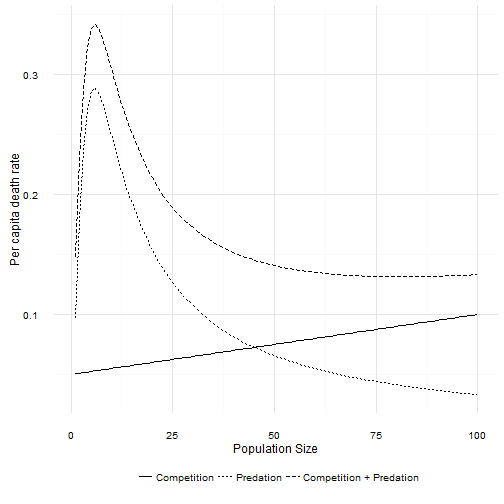
The combination of death due to intraspecific competition and death due to a Type III predator creates a non-linear response of total per capita death rates to population size. Total per capita death rate first increases as population size increases. The curve hits a maximum and then begins to decline with increasing population size just like a Type II curve. Eventually, as population size increases the per capita death due to predation asymptotes to 0. At large population sizes the death rate is again linear. If the per capita birth rate function is high enough, then a Type III predator also leads to dynamics that look very much like the logistic. How high is high enough? Unfortunately that’s not as easy to work out as it was for the Type II curve! However, as long as $b(N_{max}) > d(N_{max}) + \frac{aN_{max}}{2}$, we’ll have something that looks logistic. The per capita birth rate has to be higher than the peak in the figure above.

If that condition is not met, then there are two possibilities. First the most interesting case. The per capita birth rate intersects the per capita death rate somewhere to the right of the maximum predation rate. That point will be stable, and it corresponds to $K$ in the absence of predation. Closer to the maximum predation rate, but still to the right of it, there will be an unstable equilibrium point. This is the upper boundary of the “predator pit” created by a Type II predator. Just as in the Type II case, a population slightly larger than this point will increase to the upper stable equilibrium. A population slightly smaller will decrease towards zero. Unlike the Type II case, there is a third equilibrum point bigger than zero. This one is stable. Thus in this case there is a “floor” to the predator pit that is not extinction!

In the second case the per capita birth rate curve is below the death rate everywhere above the maximum predation point. Then there will be just one equilibrium point, and it will be the third stable point above, close to zero abundance.

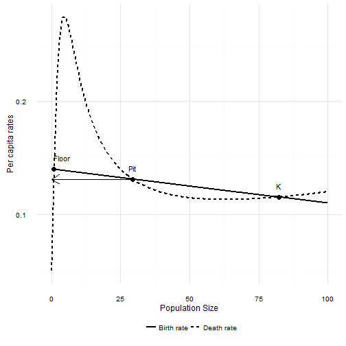
When $N$ is smaller than Pit, the death rate is larger than the birth rate and the population will decline. When $N$ is larger than Pit the death rate is lower than the birth rate and the population increases.

As with simpler predation models the logistic model turns out to be surprisingly good approximation of what happens when adding predation to the logistic model. The critical assumption is that the number of predators doesn’t change with changes in the number of the focal species.

There’s another intriguing idea to explore here. Imagine your predator is a Type III predator, and the predator pit has a floor. But you only have data on the prey. As prey abundance fluctuates around the upper equilibrium, observe how the per capita death rate varies. It is going to look quadratic. But it would look the same with a Type II predator as well! It isn’t until the prey drops past the edge of the predator pit that the difference between these two predators appears.

Even worse, the floor of the pit is at very low abundances. A time series of real, hence discrete and local, population abundances may show many zeros. This is true whether the current equilibrium is really zero or just very close to zero. Immigration into the study area could obscure the difference between the Type II and Type III predators.

I’m going to go out on a limb and predict that you won’t be able to distinguish between Type II and Type III predation on the basis of a time series of prey per capita death rates. You’ll need to observe the predator consumption rate directly at a range of prey densities, most especially including densities at low prey abundance. In practical terms that probably doesn’t matter. If you care about the prey species, all that matters is avoiding the edge of the predator pit. What happens in the pit it is less important, because the distinction between Type II and Type III disappears when dealing with populations of discrete individuals. They are both highly likely to go locally extinct once they are in the pit.