How do predators change population growth?

The logistic model of population growth includes the effects of predation. Predators are one of the factors contributing to death rates, and so if a species has any predators at all, predation is part of the logistic model. This isn’t widely appreciated. What I want to do here is ask what kinds of predation are consistent with the basic logistic model.

Start with the fundamental equation of population dynamics:

$$N' = bN - dN + I - E$$

$b$ and $d$ are per capita birth and death rates. $N'$ is the rate of change in the population. I assume $I = E = 0$ (a closed population), and divided by $N$ to convert this to a per capita rate of change.

$$\frac{N'}{N} = b\left(N\right) - d\left(N\right)$$

The logistic model when $b(N)$ and $d(N)$ are linear functions of $N$. As long as $db/dN < 0$, $dd/dN > 0$, and $b(0) > d(0)$¹ this model has a positive equilibrium point which we call $K$, the carrying capacity. Now we usually assume these changes are due to intra-specific competition. But predation causes death, so what kind of predation can be accommodated in this model without changing the fundamental dynamics?

Modelling basic predators

The simplest form of predator-prey interaction is a mass action model, where the frequency of interactions between a predator and prey are proportional to the product of their abundances. The constant of proportionality represents all kinds of processes, like the predators ability to detect the prey, pursue and capture the prey, etc. So the number of prey eaten by $P$ predators is $E = a NP$,² and dividing by $N$ to put it into our per capita growth rate equation

$$\frac{N'}{N} = b\left(N\right) - d\left(N\right) - aP$$

This leads to an interesting observation: as long as $P$ is constant, and $b(0) > d(0) + aP$, this is still the classical logistic model. $P$ can be (approximately) constant for all sorts of reasons. The generation time of the predator could be very slow compared to the prey. The predator could eat lots of other things, and so changes in the focal species abundance don’t affect the predator population very much.

One interesting observation from this addition to the logistic model: if outside forces cause $P$ to increase such that $b(0) < d(0) + aP$, then the focal species population will begin to decline exponentially towards 0.

Adding some reality

The predators above don’t have alot of behavior. In particular, they never get full and they never ignore the focal species. Both of these phenomena are well known for real predators.

Predator satiation

A real predator takes some amount of time to ‘‘handle’’ a prey item. Handling time includes the time needed to capture and subdue, consume, and digest the prey. The key assumption is that a predator can only handle one prey at a time. When prey are scarce, this doesn’t really matter. The predators time is dominated by the time spent searching for prey. But the more abundant a prey item is, the more time is spent handling instead of searching. Ultimately, the predator spends all of its time handling prey! This phenomenon sets an upper limit on the number of prey that can be consumed by a single predator.³ The resulting non-linear relationship between prey abundance and predation rate is called a Type II functional response. The basic predator model is known as a Type I functional response. The simplest Type II functional response equation is

$$E = \frac{aNP}{1+ahN}$$

The numerator is the same as the simple predator above. $aP$ is now the maximum per capita rate of death due to predation. This maximum occurs when $N = 0$. Unlike the simple predator, the per capita rate of death from predation decreases as population size increases. That actually surprised me. I mean, it’s perfectly obvious now that I’ve worked out the equation, but my intuition about how the per capita death rate changes was badly misled by the fact that the number eaten increases with population size.

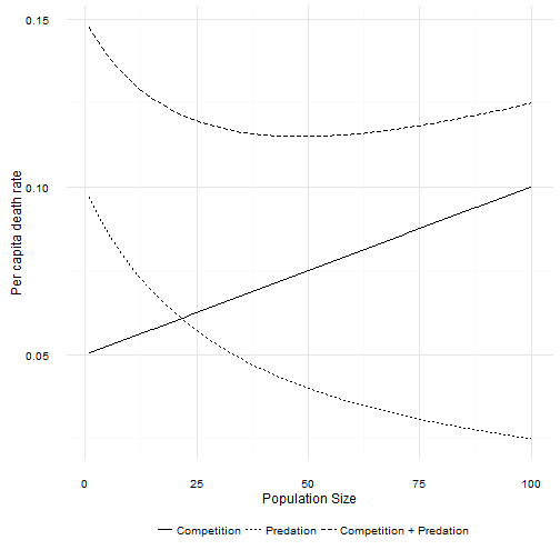
The combination of death due to intraspecific competition and death due to a Type II predator creates a non-linear response of total per capita death rates to population size. Total per capita death rate first declines as population size increases. However, as population size increases the per capita death due to predation asymptotes to 0. At large population sizes the death rate is again linear. If the per capita birth rate function is high enough, then a Type II predator also leads to dynamics that look very much like the logistic. How high is high enough? Well, as long as $b(0) > d(0) + aP$! That looks familiar …

If that condition is not met, then the focal population will decline exponentially towards zero. That is exactly the same response as with a Type I predator. However, the Type II predator creates a new possibility. The per capita death rate first decreases before increasing. If $b(0)$ is not too much smaller than $d(0) + aP$, and $db/dN$ is not too steep⁴, then there are two equilibrium points in the population. The larger of the two is the carrying capacity $K$. The new equilibrium point is lower, and occurs where the per capita death rate decreases to below the per capita birth rate. The interesting thing about this new point is that it is unstable. If the population size is just a bit larger, the population increases to $K$. If the population is a bit smaller than this point, the population decreases to 0. This new equilibrium point marks the upper edge of a predator pit.

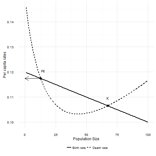
When $N$ is smaller than Pit, the death rate is larger than the birth rate and the population will decline. When $N$ is larger than Pit the death rate is lower than the birth rate and the population increases.

The logistic model turns out to be surprisingly good approximation of what happens with predation. The critical assumption is that the number of predators doesn’t change with changes in the number of the focal species.