Sampling

Generate a random sample

Once you have decided to use simple random sampling to choose your sites, how do you do it? There are two steps.

• Create or obtain a vector of all possible sampling units
• Use sample() to select the units you will use.

We’ve already done the first step. So now we look at the next step, picking our random sample. The sample() function will choose a random sample of size = n with or without replacement.

# code to be executed
sampleFrame <- as.character(1:1000)
sampleIndex <- sample(sampleFrame, size = 50, replace = TRUE)
sampleIndex

 [1] "359" "799" "114" "881" "901" "216" "922" "896" "886" "893" "421"
[12] "602" "988" "829" "894" "136" "760" "825" "687" "468" "56"  "111"
[23] "527" "997" "248" "497" "667" "321" "641" "459" "471" "902" "818"
[34] "7"   "462" "475" "968" "290" "170" "447" "891" "804" "535" "188"
[45] "216" "411" "602" "520" "632" "906"

The first argument to sample() is the sampleFrame, the vector with the ID of each sample unit. The second argument size indicates the number of units to sample. The first argument describes whether the sample is drawn with replacement or not.

So using our data.frame of Nebraska Counties, a size of 10 and without replacement:

simple_sample <- sample(sample_frame$COUNTYNAME, size = 10, replace = FALSE)
simple_sample

 [1] Nemaha     York       Wheeler    Custer     Dawes      Valley    
 [7] Banner     Dundy      Richardson Kearney   
93 Levels: Adams Antelope Arthur Banner Blaine Boone Box Butte ... York

And there you go! What’s that? Your list of 10 is different from mine? Yes, and that is expected. Computers generate random numbers from iterative algorithms that start with a “seed” value. If you do not use the same seed then the sequence of random numbers will be different. Most of the time that’s what you want. However, if you want your calculations to be exactly reproducible you need to explicitly set the seed of the random number generator. The value you give it doesn’t matter. As long as you set the seed the sequence of random numbers that follow will be exactly the same.

sample(1:1000, size = 10)

 [1] 979 431 781 153 468 638 659  76 695 594

sample(1:1000, size = 10) # different

 [1] 673 157 113 997 567 171 264 123  32 690

set.seed(3987274)
sample(1:1000, size = 10)

 [1] 877 290 236 595 307 771 414  35 486 584

set.seed(3987274)
sample(1:1000, size = 10) # same! 

 [1] 877 290 236 595 307 771 414  35 486 584

There are a few problems with our simple random sample of counties. Each county has the same probability of being selected, despite the fact that they have different areas. In effect, this means that a bit of ground in Lancaster county has a higher probability of being selected than a bit of ground in Cherry county. To get around this we need to weight the probability of choosing each county by its area. This is called a “probability proportional to size” sample. sample() has an argument called prob which takes a numeric vector. The only condition is that all the elements of this vector have to be positive.

set.seed(39858309)
sample(sample_frame$COUNTYNAME, size = 10, prob = sample_frame$area)

 [1] Knox     Sioux    Webster  Cherry   Dawes    Cuming   Frontier
 [8] Custer   Sheridan Arthur  
93 Levels: Adams Antelope Arthur Banner Blaine Boone Box Butte ... York

There is another way we might want to sample a geographical space. It’s possible that we want to choose random points within a particular area. Each spatial polygon has a “bounding box” associated with it.

bbox(counties)

        min      max
x 159215.36 900447.3
y  18672.44 359430.7

These have units of meters, which you can see by checking the projection information. Look for +units=m.

proj4string(counties)

[1] "+proj=lcc +lat_1=40 +lat_2=43 +lat_0=39.83333333333334 +lon_0=-100 +x_0=500000 +y_0=0 +datum=NAD83 +units=m +no_defs +ellps=GRS80 +towgs84=0,0,0"

So, we can pick a random point between two values using runif(), which is a random sample from a uniform distribution.

bb <- bbox(counties)
runif(1,min=bb[1,1],max=bb[1,2])

[1] 244246.5

So we can pick 100 samples in both x and y dimensions like this:

rand_points <- data.frame(x = runif(100, min=bb[1,1],max=bb[1,2]),
                          y = runif(100, min=bb[2,1],max=bb[2,2]))

Figuring out exactly where those points are can be tricky, but to make a map we need to put the coordinates into a spatialpointsDataFrame object that has the same projection information as the counties spatialPolygonsDataFrame does.

rp <- SpatialPoints(rand_points,proj4string = CRS(proj4string(counties)))
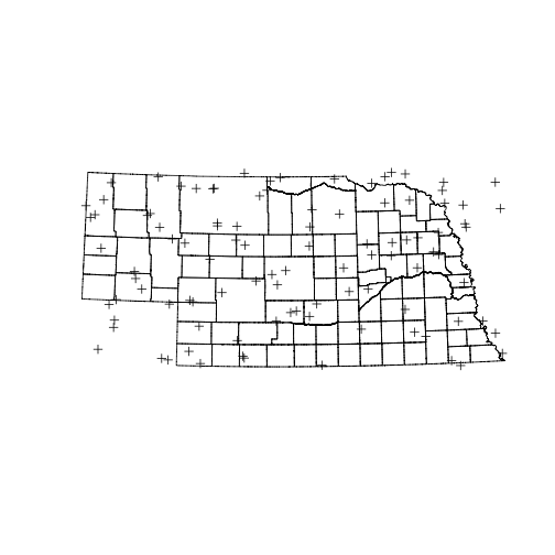
plot(counties)
plot(rp, add=TRUE)

The problem with this simple approach is obvious. Some of the points selected are outside Nebraska because the state is not a perfect match for it’s bounding box. The function over() can help here

head(over(rp, counties))

  OBJECTID FIPS_C FIPS_I FIPSST FIPSCO STPO COUNTYNAME
1     1918  31131  31131     31    131   NE       Otoe
2     1919  31165  31165     31    165   NE      Sioux
3       85  31101  31101     31    101   NE      Keith
4     2543  31159  31159     31    159   NE     Seward
5       73  31041  31041     31    041   NE     Custer
6       NA   <NA>     NA   <NA>   <NA> <NA>       <NA>
                 CNTYDISP  CNTYSHORT  CNTYSORT CNTYCATEGO CNTYACTIVE
1   Otoe County, Nebraska   OTOE, NE   NE-Otoe     County          Y
2  Sioux County, Nebraska  SIOUX, NE  NE-Sioux     County          Y
3  Keith County, Nebraska  KEITH, NE  NE-Keith     County          Y
4 Seward County, Nebraska SEWARD, NE NE-Seward     County          Y
5 Custer County, Nebraska CUSTER, NE NE-Custer     County          Y
6                    <NA>       <NA>      <NA>       <NA>       <NA>
  INDEPCITY CNTYSTAND  SEATLAT   SEATLONG NAD83UTM NAD83STATE NAD27STATE
1         N         Y 40.67667  -95.85889    26914      32104      32006
2         N         Y 42.68722 -103.88222    26913      32104      32005
3         N         Y 41.12806 -101.71917    26914      32104      32006
4         N         Y 40.90694  -97.09861    26914      32104      32006
5         N         Y 41.40194  -99.63889    26914      32104      32006
6      <NA>      <NA>       NA         NA       NA         NA         NA
  STATENAME CNTYSTARTD CNTYENDD   LASTCHGD NOTE   BOTTOM     TOP_
1  Nebraska       <NA>     <NA> 2003/02/24 <NA> 40.52273 40.78445
2  Nebraska       <NA>     <NA> 2003/02/24 <NA> 42.00050 43.00171
3  Nebraska       <NA>     <NA> 2003/02/24 <NA> 41.00268 41.39552
4  Nebraska       <NA>     <NA> 2003/02/24 <NA> 40.69784 41.04687
5  Nebraska       <NA>     <NA> 2003/02/24 <NA> 41.04622 41.74159
6      <NA>       <NA>     <NA>       <NA> <NA>       NA       NA
       LEFT_     RIGHT_
1  -96.46383  -95.70997
2 -104.05315 -103.40097
3 -102.05573 -101.24996
4  -97.36851  -96.91059
5 -100.25293  -99.20326
6         NA         NA

So overlaying counties onto the points gives us missing values for all the points outside of Nebraska. We can use this to filter our sample. That would leave us with less than 100 points. So instead we choose many more points than we want, and then randomly sample 100 from the ones that are inside Nebraska.

rand_points <- data.frame(x = runif(400, min=bb[1,1],max=bb[1,2]),
                          y = runif(400, min=bb[2,1],max=bb[2,2]))
rp <- SpatialPoints(rand_points,proj4string = CRS(proj4string(counties)))
inside <- !is.na(over(rp, counties)$OBJECTID)
rp <- rp[inside]
pick <- sample(1:length(rp), size = 100, replace = FALSE)
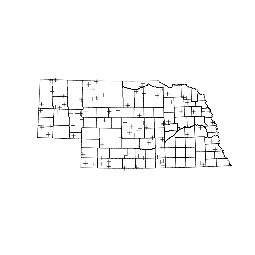
plot(counties)
plot(rp[pick], add=TRUE)

There’s another wrinkle here. The probability of picking any spot inside the state probably changes from east to west and south to north because the earth is a sphere. How much this matters probably depends on the projection in use as well as the extent over which the sample is being taken.