How to read a tab delimited file

The semester long course from Data Carpentry uses read.csv(..., sep="\t") to read tab delimited files. I’ve been using readr::read_tsv() because … well, just because! A student in my data management class (reasonably) had this question:

Will both of these essentially do the same thing or are there considerations for using one vs. the other?

So that’s a good question. The short answer is yes, they do the same thing. The longer answer is: except when they don’t! And those differences will break your code.¹

The first dataset I had the students use comes from a study of forests in India. This one is fairly clean and easy.

baser <- read.csv("http://esapubs.org/archive/ecol/E091/216/Macroplot_data_Rev.txt", sep="\t")
tidyv <- read_tsv("http://esapubs.org/archive/ecol/E091/216/Macroplot_data_Rev.txt")

## Parsed with column specification:
## cols(
##   PlotID = col_character(),
##   SpCode = col_character(),
##   TreeGirth1 = col_integer(),
##   TreeGirth2 = col_integer(),
##   TreeGirth3 = col_integer(),
##   TreeGirth4 = col_integer(),
##   TreeGirth5 = col_integer()
## )

class(baser) 

## [1] "data.frame"

class(tidyv)

## [1] "tbl_df"     "tbl"        "data.frame"

So they’re not identical because readr::read_tsv() returns a tbl_df instead of a data.frame. But the variable names are the same

all.equal(names(baser),names(tidyv))

## [1] TRUE

The main difference between the tbl_df and the data.frame is that the latter has coerced PlotID and SpCode to factors:

map_chr(baser, class)

##     PlotID     SpCode TreeGirth1 TreeGirth2 TreeGirth3 TreeGirth4 
##   "factor"   "factor"  "integer"  "integer"  "integer"  "integer" 
## TreeGirth5 
##  "integer"

and this doesn’t happen in the tbl_df

map_chr(tidyv, class)

##      PlotID      SpCode  TreeGirth1  TreeGirth2  TreeGirth3 
## "character" "character"   "integer"   "integer"   "integer" 
##  TreeGirth4  TreeGirth5 
##   "integer"   "integer"

For the most part that difference isn’t going to be noticeable, because most R functions will coerce a character vector to a factor if a factor is what they want. So, if you have nice clean data then you’ll get more or less the same thing, or with differences that can mostly be ignored.²

The second tab delimited dataset the students used comes from a comparative analysis of mammal life histories.³ It uses some non-standard representations of missing values too.

baser <- read.csv("http://esapubs.org/archive/ecol/E084/093/Mammal_lifehistories_v2.txt", sep="\t", na.strings = c("-999","-999.00"))
tidyv <- read_tsv("http://esapubs.org/archive/ecol/E084/093/Mammal_lifehistories_v2.txt", na = c("-999","-999.00"))

## Parsed with column specification:
## cols(
##   order = col_character(),
##   family = col_character(),
##   Genus = col_character(),
##   species = col_character(),
##   `mass(g)` = col_double(),
##   `gestation(mo)` = col_double(),
##   `newborn(g)` = col_double(),
##   `weaning(mo)` = col_double(),
##   `wean mass(g)` = col_double(),
##   `AFR(mo)` = col_double(),
##   `max. life(mo)` = col_integer(),
##   `litter size` = col_double(),
##   `litters/year` = col_double(),
##   refs = col_number()
## )

I have a love/hate relationship with one feature of readr functions – the messages describing what the function did. Great for developing an analysis. Less great for reporting. This dataset demonstrates one of the other big differences between base::read.csv() and readr::read_tsv(). The latter doesn’t do anything to column names, while read.csv() by default checks the column names to make sure they don’t contain any nasty bits. You can turn this behavior off. So:

all.equal(names(baser), names(tidyv))

## [1] "9 string mismatches"

names(tidyv)

##  [1] "order"         "family"        "Genus"         "species"      
##  [5] "mass(g)"       "gestation(mo)" "newborn(g)"    "weaning(mo)"  
##  [9] "wean mass(g)"  "AFR(mo)"       "max. life(mo)" "litter size"  
## [13] "litters/year"  "refs"

The offending characters are the slash, spaces and parentheses. For the most part you can actually work with these in R code by surrounding them with back ticks:

mean(tidyv$`mass(g)`, na.rm = TRUE)

## [1] 407701.4

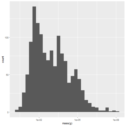
One consequence of this is that axis labels are nice straight away:

ggplot(tidyv, aes(x=`mass(g)`)) + geom_histogram() + 
  scale_x_log10()

## `stat_bin()` using `bins = 30`. Pick better value with `binwidth`.

## Warning: Removed 89 rows containing non-finite values (stat_bin).

I’m sure there are places where the back ticks won’t work, and I find them kind of … kludgy. But that might be just a bit curmudgeonly on my part. In case you do need to fix them, there’s an easy fix:

names(tidyv) <- make.names(names(tidyv))
all.equal(names(baser), names(tidyv))

## [1] TRUE

Or you could go the other way and tell read.csv() not to mess with the names:

baser <- read.csv("http://esapubs.org/archive/ecol/E084/093/Mammal_lifehistories_v2.txt", sep="\t", na.strings = c("-999","-999.00"), check.names = FALSE)
names(baser)

##  [1] "order"         "family"        "Genus"         "species"      
##  [5] "mass(g)"       "gestation(mo)" "newborn(g)"    "weaning(mo)"  
##  [9] "wean mass(g)"  "AFR(mo)"       "max. life(mo)" "litter size"  
## [13] "litters/year"  "refs"

On the whole, I can’t see much difference between the two approaches. If you (or your collaborators) prepare tidy data with best practices, you’ll rarely see a difference. But if you use #otherpeoplesdata a lot, then pick one and stick to it. That won’t solve all your data importing woes, but at least you won’t inflict unexpected ones on yourself by forgetting what your data import function does!