The sex ratio of chickens
I got the following email the other day
Im trying to find the answer to a pretty simple question, but Im having a hard time finding a reputable source online, so I Googled “best ornithology schools” and you all popped up! Im wondering if the sex ratio for egg-laying chickens is about equal, 1 male chick : 1 female chick born.
Obviously a fan! I tried the same search and I must say we didn’t exactly pop to the top.
I searched ‘sex ratio chickens’ and the first link was Hays (1945). From The American Naturalist no less, so a peer reviewed journal and a credible source. In the introduction he summarizes a range of previous sources with estimates varying from 48.77 \% males to 51.38 \% males. So approximately 50/50. In his own work (which is behind a paywall so not publicly available) he reports 49.7 \% males. His methods were
In the ten-year period from 1935 to 1944 a total of 39 pure- bred Rhode Island Red females mated to pure-bred Rhode Island Red males qualified for study. Each female had a perfect record in fertility and hatchability and produced ten or more chicks during March and April
This is 1945, so statistics are largely absent. He does suggest that the standard error of the difference between yearly sex ratios and 50 \% is 1.42. I think that’s just treating each year as a single observation. But the data are given.
| Year | # of Dams | # of Male Chicks | # of Female Chicks | Sex not determined |
|---|---|---|---|---|
| 1944 | 8 | 70 | 78 | 9 |
| 1943 | 4 | 43 | 45 | 9 |
| 1942 | 0 | NA | NA | NA |
| 1941 | 4 | 51 | 47 | 3 |
| 1940 | 6 | 92 | 85 | 5 |
| 1939 | 5 | 50 | 48 | 10 |
| 1938 | 3 | 29 | 28 | 3 |
| 1937 | 2 | 22 | 22 | 4 |
| 1936 | 3 | 21 | 34 | 14 |
| 1935 | 4 | 54 | 51 | 4 |
So treating each year as a normally distributed observation I get
sexratio <- with(table1, 100 * Males / (Females + Males))
sd(sexratio - 50, na.rm = TRUE) / sqrt(9)
## [1] 1.45542t.test(sexratio - 50)##
## One Sample t-test
##
## data: sexratio - 50
## t = -0.63463, df = 8, p-value = 0.5434
## alternative hypothesis: true mean is not equal to 0
## 95 percent confidence interval:
## -4.279855 2.432553
## sample estimates:
## mean of x
## -0.9236509So I get a slightly different standard error, but either way it isn’t significantly different from 50 %. However this is ignoring a huge amount of information in this data. For example, one thing that’s cool is the variation between years.
library(lme4)## Loading required package: Matrix
## Loading required package: methodsyear.model <- glmer(cbind(Males,Females)~1 + (1|Year), data = table1, family=binomial)
summary(year.model)## Generalized linear mixed model fit by maximum likelihood (Laplace
## Approximation) [glmerMod]
## Family: binomial ( logit )
## Formula: cbind(Males, Females) ~ 1 + (1 | Year)
## Data: table1
##
## AIC BIC logLik deviance df.resid
## 52.5 52.9 -24.2 48.5 7
##
## Scaled residuals:
## Min 1Q Median 3Q Max
## -1.7018 -0.1485 0.1845 0.3634 0.6179
##
## Random effects:
## Groups Name Variance Std.Dev.
## Year (Intercept) 0 0
## Number of obs: 9, groups: Year, 9
##
## Fixed effects:
## Estimate Std. Error z value Pr(>|z|)
## (Intercept) -0.01379 0.06781 -0.203 0.839So same conclusion as before. The intercept is not significantly different from 0, which is what we expect for 50/50 sex ratio. In addition, there’s no evidence of significant variation between years. The estimated random effect variance is zero.
Hays also has a table of data for 11 hens with complete records of sex of chick. The sex ratio there extends from 22 % up to 65 %! So repeating the same thing
ind.model <- glmer(cbind(Males,Females)~1 + (1|Hen), data = table2, family=binomial)
summary(ind.model)
## Generalized linear mixed model fit by maximum likelihood (Laplace
## Approximation) [glmerMod]
## Family: binomial ( logit )
## Formula: cbind(Males, Females) ~ 1 + (1 | Hen)
## Data: table2
##
## AIC BIC logLik deviance df.resid
## 71.7 72.5 -33.9 67.7 9
##
## Scaled residuals:
## Min 1Q Median 3Q Max
## -0.70263 -0.17421 -0.02554 0.04426 0.94412
##
## Random effects:
## Groups Name Variance Std.Dev.
## Hen (Intercept) 0.7791 0.8827
## Number of obs: 11, groups: Hen, 11
##
## Fixed effects:
## Estimate Std. Error z value Pr(>|z|)
## (Intercept) 0.2053 0.2978 0.689 0.491Again, the intercept is not significantly different from zero, so across the entire population the average sex ratio is not different from 50/50. However here we do see a non-zero variance between hens. Individual hens may have sex ratios that deviate from 50/50. It’s a bit hard to interpret that standard deviation because it is on a log-odds scale.
Imagine you are ordering chicks ‘straight run’, which means without sexing. This is the cheapest way to get chicks because the expertise to sex chicks at a young age is expensive. You want 4 hens, so you decide to order 8 chicks. With a 50/50 sex ratio you’ll get 4 hens, right?
Wrong! You can get any number of hens between 0 and 8! 4 is just the most likely outcome. In fact, nearly 4 out of 10 orders you’ll get less than 4 hens. Of course, you could also do better; in 4 out of 10 orders you’ll get more than 4 hens. The probabilities of each outcome are
binomial_probs = data.frame(hens=0:8,
                            d = dbinom(0:8, 8, 0.5),
                            p = pbinom(0:8, 8, 0.5))

knitr::kable(binomial_probs, digits = 2)| hens | d | p |
|---|---|---|
| 0 | 0.00 | 0.00 |
| 1 | 0.03 | 0.04 |
| 2 | 0.11 | 0.14 |
| 3 | 0.22 | 0.36 |
| 4 | 0.27 | 0.64 |
| 5 | 0.22 | 0.86 |
| 6 | 0.11 | 0.96 |
| 7 | 0.03 | 1.00 |
| 8 | 0.00 | 1.00 |
However, that assumes that there is no variation among hens, which we know is false. I can simulate data from the fitted model to see if this variation makes a difference to the probability of getting less than 4 hens.
hens <- 1000
clutchsize <- 8
clutches <- matrix(NA, nrow = hens, ncol = 2)
mean_p <- ind.model@beta
var_p <- as.numeric(vcov(ind.model)) # uncertainty in p
var_ind <- ind.model@theta^2
logodds <- rnorm(hens, mean = mean_p, sd = sqrt(var_p + var_ind))
# convert to probability
p <-  1 / (1 + exp(-logodds))
males <- rbinom(hens, size = clutchsize, p = p)

library(ggplot2)
## Warning: package 'ggplot2' was built under R version 3.2.4binomial_probs$freq <- binomial_probs$d * hens
gg <- ggplot(as.data.frame(males),aes(x=males)) + geom_bar() + geom_line(data=binomial_probs, mapping=aes(x=hens, y=freq))
gg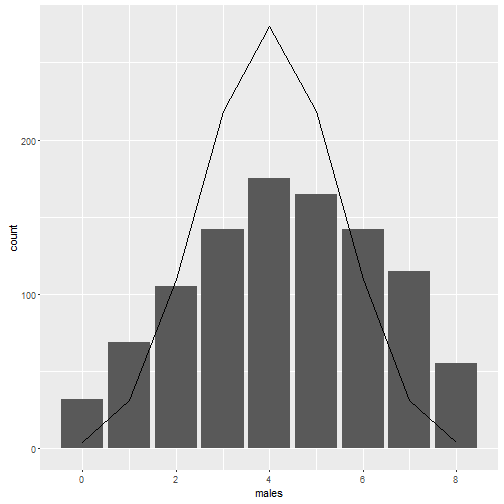
So by including the between hen variation we end up with 34 % of orders having more than 4 females. This is about the same as without the between individual variation. However, there is a greater chance of getting 1 or 0 hens (7 or 8 males) in the order.
Not sure what the takehome is here. Randomness is two faced?